# Home

Inverse Finance powered Analytics

{% hint style="info" %}
This website is currently in construction. Please bear with us and don't hesitate to[ reach out to the AWG in discord for any questions.](https://discordapp.com/channels/790157548845924352/848225246443470848)
{% endhint %}

On March 9, 2022, Inverse Finance holders voted for the launch of the **Analytics Working Group** (AWG) within the DAO to support our growth, define further and execute the Data Strategy as per [proposal 7 of Mills era.](https://www.inverse.finance/governance/proposals/mills/7)

<figure><img src="https://4269815422-files.gitbook.io/~/files/v0/b/gitbook-x-prod.appspot.com/o/spaces%2FGc9mnST31tkU3h2NNgSL%2Fuploads%2FhqaO6biJv9OQc4VUCtwg%2FUntitled%20design(1).png?alt=media&amp;token=eb02739f-b9e2-4fc2-9888-3459f27e5887" alt="" width="375"><figcaption></figcaption></figure>

The main goal of the AWG is to enable members and users to seamlessly **access the data of their interest**, and to be able to **use it in the environment of their choice**. Because of all the tools and range of skills involved in the space, it is not always an easy task to do so.

Within that perspective, the Analytics Working Group provides our members and users with the following :&#x20;

[**​Dynamic Dashboards :**](/products/inverse-watch) based on **PostgreSQL** queries and relying on **an in house** flexible environment (forked from Redash), allowing on-the-fly analysis and CSVs extractions for specific or urgent needs ;​

[**GraphQL endpoints :**](/products/inverse-subgraphs) based on **The Graph** enabling to index on-chain events as soon as they happen and making the protocol information accessible to everyone through a **GraphQL endpoint ;**&#x200B;

[**Alert and Social notifications :**](/products/inverse-alerts) thanks to our extensive infrastructure we are able to display beautiful notifications and alerts in Discord or Twitter, from any data source.

Inverse Watch is a platform created by the AWG with the goal of centralizing its services, and make data analytics tasks less repetitive and more efficient in order to better serve the DAO.


# Governance

This page lists the governance proposals empowering the Analytics Working Group to carry its tasks and duties.

## **Proposal 7**

{% embed url="<https://www.inverse.finance/governance/proposals/mills/7>" %}

## **Proposal 25**

{% embed url="<https://www.inverse.finance/governance/proposals/mills/25>" %}

## **Proposal 52**

{% embed url="<https://www.inverse.finance/governance/proposals/mills/52>" %}

## **Proposal 107**

{% embed url="<https://www.inverse.finance/governance/proposals/mills/107>" %}

## **Proposal 147**

## <https://www.inverse.finance/governance/proposals/mills/147>

## **Proposal 189**

## <https://www.inverse.finance/governance/proposals/mills/189>


# Inverse Alerts

InverseAlerts is a robust and innovative bot based on the inverse.watch platform designed to deliver real-time blockchain market information to the public via Twitter. The primary objective of this bot is to democratize the complex realm of blockchain information and render it accessible, thereby making market movements and trends readily comprehensible for the general public.

<div data-full-width="true"><figure><img src="https://4269815422-files.gitbook.io/~/files/v0/b/gitbook-x-prod.appspot.com/o/spaces%2FGc9mnST31tkU3h2NNgSL%2Fuploads%2FsHfsk7NfYDdJHFcuvsjK%2Fimage.png?alt=media&amp;token=2822e85c-ea61-49a6-954a-80100457e57b" alt="" width="300"><figcaption><p>Follow @InverseAlerts and stay informed</p></figcaption></figure></div>

The bot leverages the power of blockchain's transparency by tracking and analyzing complex on-chain activities. It identifies significant market moves, patterns, and trends on various blockchain networks and swiftly broadcasts this information on Twitter, making it easily accessible to anyone, anywhere. This on-demand, readily accessible information significantly aids in risk management by enabling users to make informed decisions and act swiftly based on market dynamics.

Furthermore, InverseAlerts bolsters the transparency of blockchain transactions by delivering these insights to the public domain. The democratization of this information goes a long way in educating individuals about blockchain activities, thus promoting blockchain literacy and stimulating informed participation. The real-time, automated nature of the bot ensures that users are always kept abreast of the most current trends, fostering a sense of trust, confidence, and empowerment among users.

[Follow us to stay informed !](https://twitter.com/InverseAlerts)


# Inverse Chatbot

The Inverse Flaskbot is a sophisticated Discord bot designed specifically to support the Inverse Finance DAO community. With its advanced data processing and AI capabilities, it serves as a pivotal tool in facilitating access to information, enhancing community engagement, and supporting content creation. By integrating a comprehensive set of machine learning and AI technologies, the Flaskbot provides a seamless experience for users to query finance-related documentation and generate creative visuals, aiding contributors in social media and web development endeavors.

**Infrastructure and Key Technologies**

The Flaskbot’s robust infrastructure is built upon a selection of cutting-edge technologies:

* **Machine Learning Libraries (Ollama & Torch)**: These are the backbone for the bot's AI functionalities, allowing for complex data analysis and processing tasks.
* **Natural Language Processing (Diffusers & Transformers)**: These tools enable the bot to understand and generate human-like text responses, making interactions intuitive.
* **Image Generation (Open Source Models & Stablediffusion Pipeline)**: Powers the bot's ability to create images from textual descriptions, catering to the creative needs of the community.
* **Adaptive AI Model Integration**: With the flexibility to switch between self-hosted models and OpenAI's cloud services, the Flaskbot ensures optimal performance for both text and image generation tasks, depending on resource availability and specific user requirements.

This technology stack ensures that the Flaskbot is not just a chatbot but a comprehensive tool for information retrieval and creative content generation, tailored to the needs of the Inverse Finance DAO community.


# /doc

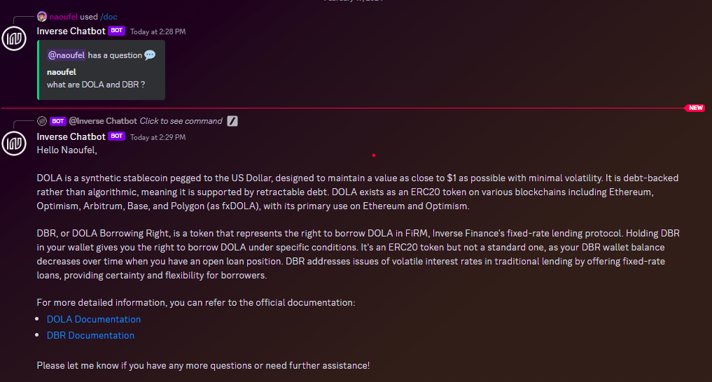
The `/doc` command is a cornerstone feature of the Inverse Flaskbot, designed to empower the Inverse Finance DAO community by providing quick and easy access to a vast repository of financial documentation. Whether it's detailed information about tokens, protocols, or lending practices, the `/doc` command ensures that community members can find accurate and relevant information instantly.

**How to Use the `/doc` Command**

1. **Initiate a Query**: Simply type `/doc` followed by your specific question or keywords in any Discord channel where the Flaskbot is active. For example: `/doc what are DOLA and DBR ?`
2. **Review the Bot's Response**: The Flaskbot will quickly sift through the documentation and return a concise, relevant answer to your query.

<figure><img src="https://4269815422-files.gitbook.io/~/files/v0/b/gitbook-x-prod.appspot.com/o/spaces%2FGc9mnST31tkU3h2NNgSL%2Fuploads%2FI7mXOcJ9rc6nSHWwopys%2Fimage.png?alt=media&amp;token=aa113691-74bf-480e-ae46-ef70beefab01" alt=""><figcaption></figcaption></figure>

3. **Iterate for More Details**: If necessary, refine your query with additional keywords to narrow down the search results for more precise information.


# /imagine

The `/imagine` command within the Inverse Flaskbot toolkit is a revolutionary feature designed for the Inverse Finance DAO community, particularly benefiting contributors focused on marketing, social media outreach, and web design. It provides an intuitive way to generate images that align with the DAO's unique brand identity, incorporating specific color schemes and thematic elements that resonate with the community's vision.

**Crafting Images that Reflect the DAO's Identity**

The Inverse Finance DAO's brand identity is characterized by its distinctive color palette of seafoam green, dark and light purples, and its iconic pixel invaders, all wrapped in a graffiti cypherpunk style. The `/imagine` command is perfectly suited to creating visuals that embody these elements, offering an endless stream of creativity for digital content that stands out.

**How to Use the `/imagine` Command for Brand-Themed Visuals**

1. **Compose Your Description**: When using the `/imagine` command, craft a prompt that encapsulates the essence of the DAO's brand. Mention the specific colors, themes, and styles that should be featured. \
   For example: `/imagine` a vibrant cityscape at night, illuminated by seafoam green and purple lights, pixel invaders tagging buildings with graffiti in a cypherpunk style `height: 1024` `width: 1792`

<figure><img src="https://4269815422-files.gitbook.io/~/files/v0/b/gitbook-x-prod.appspot.com/o/spaces%2FGc9mnST31tkU3h2NNgSL%2Fuploads%2FfTezqzVjpf3NM8jYr7wi%2Fimage.png?alt=media&amp;token=24897f78-d6a6-4e92-8f9d-5282c950904c" alt=""><figcaption><p>Ouput of the prompt</p></figcaption></figure>

3. **Receive and Review Your Image**: The Flaskbot processes your detailed prompt and generates an image that brings your vision to life. This image will be shared in the Discord chat, providing you with a visual asset that perfectly aligns with the DAO's branding.
4. **Refine Your Request**: Don't hesitate to experiment with different combinations of themes, colors, and elements. The more specific you are with your descriptions, the closer the generated images will be to your envisioned outcome.

#### Tips for Maximizing the Impact of the `/imagine` Command

* **Be Detailed in Your Descriptions**: The effectiveness of the AI in generating your desired image heavily relies on the specificity and clarity of your prompt. Include details about the ambiance, key elements, and the overall mood you aim to capture.
* **Incorporate Brand Elements**: Always weave in the DAO's core brand elements — seafoam green, dark and light purples, pixel invaders, and a graffiti cypherpunk style — to maintain a consistent and recognizable brand identity across all visuals.
* **Utilize for Diverse Content Creation**: Think beyond social media posts. Use the `/imagine` command to create visuals for blog posts, website banners, promotional materials, and more, ensuring a cohesive and engaging brand presence across all platforms.

The `/imagine` command is a potent tool in the Inverse Finance DAO's arsenal, empowering community members to generate visually compelling content that echoes the DAO's ethos and aesthetic preferences. By harnessing this feature, the community can ensure that every piece of content not only captures attention but also reinforces the unique identity of the Inverse Finance DAO across the digital landscape.


# /data

The `/data` command is an innovative feature of the Inverse Flaskbot designed to provide the Inverse Finance DAO community with direct access to a wealth of financial data and insights. By leveraging advanced AI agents, this command queries our extensive databases to fetch precise information, analytics, and insights, thereby supporting data-driven decision-making within the DAO.

**How to Use**

To utilize the `/data` command effectively, follow these steps:

1. **Invoke the Command**: Type `/data` followed by your specific query in any Discord channel where the Inverse Flaskbot is active. Ensure your query is clear and concise to facilitate accurate data retrieval.
2. **Wait for the Bot's Response**: The Flaskbot processes your query using AI agents and returns the requested data directly in the chat. The response will include key insights and information relevant to your query, formatted for easy comprehension.
3. **Refine Your Query if Needed**: If the initial response doesn't fully meet your needs, consider refining your query with additional details or keywords and repeat the process.

**Example**

* **User**: `/data current liquidity of DOLA in DeFi protocols`
* **Bot Response**: "The current liquidity of DOLA across DeFi protocols is approximately $X,XXX,XXX. For more detailed breakdowns, please refer to \[link]."


# /graph

The `/graph` command is a sophisticated feature within the Inverse Flaskbot toolkit, designed to make GraphQL data fetching intuitive and accessible for the Inverse Finance DAO community. Unlike traditional GraphQL queries that require specific syntax, the `/graph` command understands natural language queries. This functionality allows users to request complex data sets from subgraphs without needing detailed knowledge of GraphQL query structure, significantly simplifying data access for community members.

**How to Use**

Fetching data with the `/graph` command is straightforward and user-friendly:

1. **Invoke the Command**: Type `/graph` followed by your query in natural language in any Discord channel where the Inverse Flaskbot is active. Clearly state what data you are looking for in a concise manner. Example : `/graph Show me the total value locked in Inverse Finance`
2. **Bot Processes Your Query**: The Flaskbot interprets your natural language query, formulates a corresponding GraphQL query, and fetches the requested data from the appropriate subgraph.
3. **Receive Your Data**: The bot will reply with the data you requested, presented in a clear and concise format directly in the Discord chat.
4. **Refine Your Query if Necessary**: If the initial response doesn't fully satisfy your request, you can refine your query with additional details or keywords and repeat the proc

This approach to data fetching not only democratizes access to complex data sets but also enhances the overall user experience by allowing more intuitive interaction with the Inverse Flaskbot. By catering to natural language queries, the `/graph` command ensures that even users without technical backgrounds can effectively engage with and benefit from the wealth of data available through the DAO's subgraphs.


# Inverse Subgraphs

Subgraphs are open APIs that index blockchain data in a highly structured and accessible manner, enabling dApps and other users to query that data efficiently. They form an integral part of The Graph, a decentralized protocol for indexing and querying data from blockchains.

<figure><img src="https://4269815422-files.gitbook.io/~/files/v0/b/gitbook-x-prod.appspot.com/o/spaces%2FGc9mnST31tkU3h2NNgSL%2Fuploads%2Fe1OKA3Y44QWUBnjddV27%2Fimage.png?alt=media&amp;token=4f274027-fb59-4faa-aab6-e5a81fc5cc95" alt="" width="563"><figcaption></figcaption></figure>

Inverse-Subgraph is a specialized subgraph developed to primarily index data from the deprecated lending protocol known as Frontier. Even though Frontier is no longer in active use, the historical data indexed and stored by Inverse-Subgraph can provide valuable insights into past trends, operations, and user behavior. This information can be instrumental for understanding and improving upon past practices, as well as aiding in the creation of new strategies and products.

{% embed url="<https://thegraph.com/explorer/subgraphs/78kqSQgaXhtfypzCE1uoB6tTCdgynowp5574ADL6RQrS?chain=mainnet&view=Playground>" %}
See on mainnet
{% endembed %}

Inverse-Governance-Subgraph, on the other hand, is designed to index data from the Inverse DAO's governance model and the latest Fixed Rate Market lending protocol, FiRM. By tracking and storing all governance-related activities, this subgraph provides transparency and accountability, key aspects of any decentralized governance model. The indexing of FiRM data aids in monitoring its functioning and detecting any patterns or anomalies that may occur, thereby providing a robust risk management mechanism.

{% embed url="<https://thegraph.com/explorer/subgraph?id=EDN34txo8wRceZvye8PkGANsSuf3XUQseG1eWrQiirma&view=Indexers>" %}
See on mainnet
{% endembed %}

Having subgraphs for the Inverse DAO is of immense value. They allow the DAO to structure its blockchain data effectively, making it easily accessible and queryable. This enhances the transparency, efficiency, and data utilization capacity of the DAO, promoting better governance and informed decision-making. Moreover, subgraphs can improve the performance of the DAO's dApps by enabling them to retrieve necessary data rapidly and accurately.


# Inverse Watch

Inverse Watch is an innovative product developed by the Inverse DAO Analytics Working Group. Designed to deliver comprehensive data analysis and alerting services, it equips stakeholders with the knowledge necessary to make informed decisions. Inverse Watch has positioned itself as a reliable source of transparent information, striving to deliver clear insights based on accurate and real-time data.

<figure><img src="https://4269815422-files.gitbook.io/~/files/v0/b/gitbook-x-prod.appspot.com/o/spaces%2FGc9mnST31tkU3h2NNgSL%2Fuploads%2F2kh7LPOfrTn1cAHexaU7%2Fimage.png?alt=media&amp;token=f90d478b-e656-4ce1-9656-8b351387f8f3" alt="" width="563"><figcaption><p>Inverse.Watch Home</p></figcaption></figure>

This sophisticated tool has been built leveraging Redash, an open-source platform for teams to query, visualize and collaborate around data. Redash has been integrated with a range of functionalities specific to the Web3 environment.

Inverse Watch facilitates its users to monitor and analyze a wide array of blockchain activities. By integrating its systems with Twitter and Discord, it disseminates alerts and reports across these platforms, ensuring that information reaches users swiftly and conveniently. For Twitter, these reports manifest as tweet alerts about significant market movements and trends, while on Discord, the bot channels comprehensive reports for community members to analyze and discuss.

<figure><img src="https://4269815422-files.gitbook.io/~/files/v0/b/gitbook-x-prod.appspot.com/o/spaces%2FGc9mnST31tkU3h2NNgSL%2Fuploads%2F1tQV06H8Um2guZhjkdkh%2Fimage.png?alt=media&amp;token=1dd42d5e-cabd-4cf8-9845-3ae004378417" alt="" width="563"><figcaption><p>Asset Scoring Model</p></figcaption></figure>

A significant feature of Inverse Watch is its capacity to render complex blockchain information accessible to the general public. By democratizing this data, it not only improves transparency but also enables individuals to actively participate in blockchain activities. Whether you're an experienced trader seeking detailed analytics or a newcomer looking for a friendly introduction to blockchain data, Inverse Watch provides an invaluable tool for navigating the ever-evolving landscape of decentralized finance.


# Quickstart

### 1. Write A Query

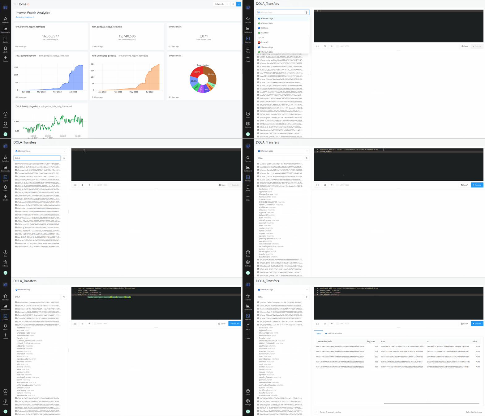
Let's explore how to write a query: **click on “Create” in the navigation bar, and then choose “Query”**. See the [Creating and Editing Queries](https://docs.inverse.watch/user-guide/queries/creating-and-editing-queries) for detailed instructions on how to write queries.

<figure><img src="https://4269815422-files.gitbook.io/~/files/v0/b/gitbook-x-prod.appspot.com/o/spaces%2FGc9mnST31tkU3h2NNgSL%2Fuploads%2FCGnQgfq5uo1JmYZBVK1m%2Fwriting_a_query.gif?alt=media&amp;token=4ce656fe-7543-483a-95ca-bb8d995b9b00" alt=""><figcaption><p>write a query</p></figcaption></figure>

### 2. Add Visualizations&#x20;

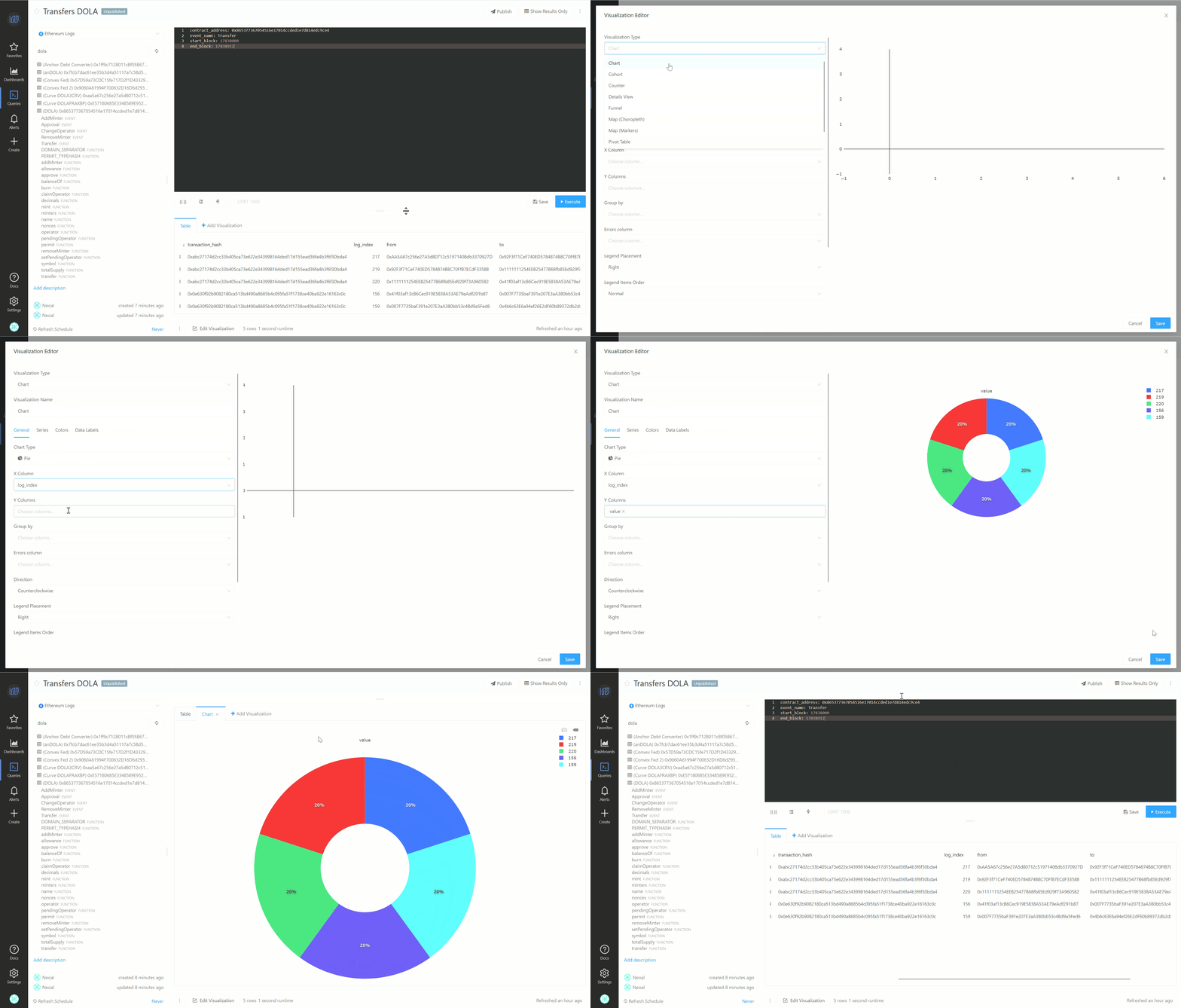
By default, your query results (data) will appear in a simple table. Visualizations are much better to help you digest complex information, so let’s visualize your data. The application supports [multiple types of visualizations](https://docs.inverse.watch/user-guide/visualizations/visualizations-types) so you should find one that suits your needs.

Click the “New Visualization” button just above the results to select the perfect visualization for your needs. You can view more detailed instructions [here](https://docs.inverse.watch/user-guide/visualizations/visualizations-how-to).

<figure><img src="https://4269815422-files.gitbook.io/~/files/v0/b/gitbook-x-prod.appspot.com/o/spaces%2FGc9mnST31tkU3h2NNgSL%2Fuploads%2FNU16yRiOe2MfosFbincD%2Fadd_visualization.gif?alt=media&amp;token=0734fa20-77f0-4d0b-9f71-420e839a8397" alt=""><figcaption><p>add visualizations</p></figcaption></figure>

### 3. Create Dashboard

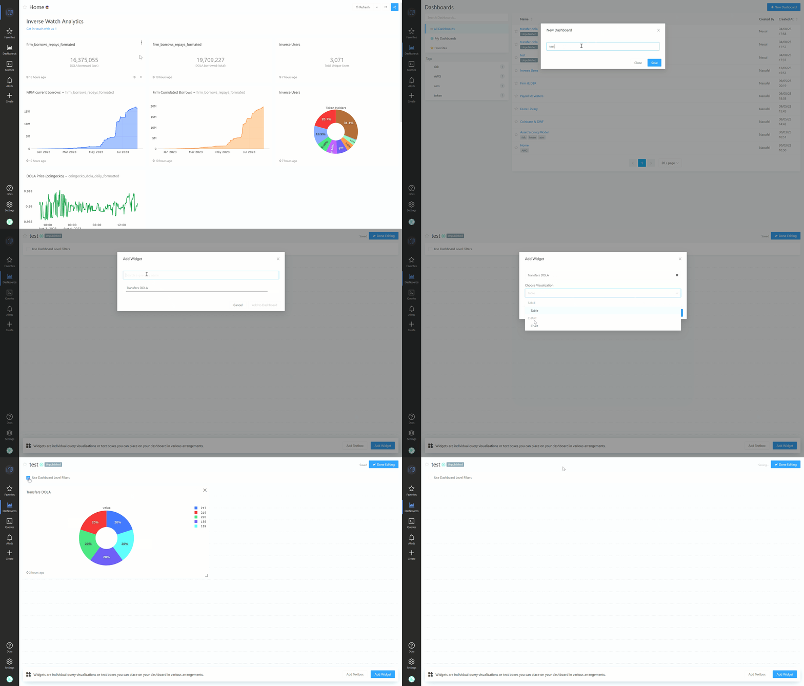
You can combine visualizations and text into thematic & powerful dashboards. Add a new dashboard by clicking on “Create” in the navigation bar, and then choose “Dashboard”. Dashboards are visible for your team members or they can be shared publicly. For more details, [click here](https://docs.inverse.watch/user-guide/dashboards/creating-and-editing-dashboards).

<figure><img src="https://4269815422-files.gitbook.io/~/files/v0/b/gitbook-x-prod.appspot.com/o/spaces%2FGc9mnST31tkU3h2NNgSL%2Fuploads%2FzMZ3Y1CZe9C3wKl7ZKY6%2Fcreate_dashboard.gif?alt=media&amp;token=85d12b13-ec7a-46e1-a17d-b9fde3d0b7d2" alt=""><figcaption><p>create Dashboard</p></figcaption></figure>


# Alerts


# Setting Up an Alert

The application alerts notify you when a field returned by a [Schedule a Query](https://docs.inverse.watch/user-guide/queries/how-to-schedule-a-query) meets a threshhold. Use them to monitor your business. Or integrate them with tools like Zapier or IFTTT to kickoff workflows such as user on-boarding or support tickets. Alerts complement scheduled queries, but their criteria are checked after every execution.

A query schedule is not required but is *highly recommended* for alerts. If you add an alert to a non-scheduled query you will be notified only if a user executes the query manually and the alert criteria are met.

{% hint style="warning" %}
A query schedule is not required but is *highly recommended* for alerts. If you add an alert to a non-scheduled query you will be notified only if a user executes the query manually and the alert criteria are met.
{% endhint %}

{% hint style="warning" %}
Alerts don’t work for queries with parameters.
{% endhint %}

To see a list of current Alerts, click **Alerts** on the navbar. By default, they are sorted in reverse chronological order by the **Created At** column. You can reorder the list by clicking the column headings.

* **Name** shows the string name of each alert. You can change this at any time.
* **Created By** shows the user that created this Alert.
* **State** shows whether the Alert status is `UNKNOWN`, `TRIGGERED`, or `OK`.

<figure><img src="https://4269815422-files.gitbook.io/~/files/v0/b/gitbook-x-prod.appspot.com/o/spaces%2FGc9mnST31tkU3h2NNgSL%2Fuploads%2FASu8K8tOjm0HxKx6ggLI%2FAlerts_page.gif?alt=media&amp;token=2ab3c61b-d3f3-4334-8d70-7a032718a35f" alt=""><figcaption></figcaption></figure>

### 1. Usage

Click the **Create** button in the navbar and then click **New Alert**.

Search for a target query. If you don’t see the one you want, make sure it is published and does not use parameters.

Use the settings panel to configure your alert.

* The **Value column** dropdown controls which field of your query result will be evaluated.
* The **Condition** dropdown controls the logical operation to be applied.
* The **Threshold** text input will be compared against the *Value column* using the *Condition* you specify.

<figure><img src="https://4269815422-files.gitbook.io/~/files/v0/b/gitbook-x-prod.appspot.com/o/spaces%2FGc9mnST31tkU3h2NNgSL%2Fuploads%2Fw633rOEp0lmV5ZqQzYwj%2Fcreate_alert.gif?alt=media&amp;token=502f5c9d-8410-4785-8140-3287e3d2f925" alt=""><figcaption></figcaption></figure>

{% hint style="info" %}
If a target query returns multiple records, the application Alerts only see the first one. As you change the Value Column setting, the current value of that field in the top row is shown beneath it.
{% endhint %}

Next, adjust how many notifications to receive while your alert is triggered. There are three options:

* **Just Once until back to normal:** means a notification will fire any time the alert status changes from `OK` to `TRIGGERED`.
* **Each time alert is evaluated until back to normal:** means a notification will fire whenever the alert status is `TRIGGERED` regardless of its status as of the previous evaluation.
* **Each time alert is evaluated for each row in the result**: This means a notification will fire for every individual row in the alert evaluation result that meets the criteria for being TRIGGERED. Regardless of the status of other rows or the previous evaluation of the same row, a unique notification will be generated for each row that is currently in a TRIGGERED state. This choice allows for granular notifications based on each specific row, ensuring that no triggering row goes unnoticed.
* **At most every ... when alert is evaluated:** lets you set a minimum interval between notifications. It splits the difference between *Just Once* and *Each time alert is evaluated*. This choice lets you avoid notification spam for alerts that trigger often.

Regardless of which notification setting you pick here, you will receive a notification whenever the status goes from `OK` to `TRIGGERED` or from `TRIGGERED` to `OK`. The schedule settings above only impact how many notifications you will receive if the status remains `TRIGGERED` from one execution to the next.

Finally, pick a **Template**. The **default template** is a message with links to the Alert configuration screen and the Query screen.

Many users will want to include more specific information about the Alert. To do this you can [Customize The Alert Template](https://docs.inverse.watch/user-guide/alerts/customize-alert-template).

When you’re finished, click **Create Alert** and then choose an [Alert Destination](https://redash.io/help/user-guide/alerts/creating-new-alert-destination). If you skip this step you will not be notified when the alert is triggered.

![](https://redash.io/assets/images/docs/gitbook/alert_destination.png)

#### i. Muting Alerts

You can temporarily mute an alert’s notifications without deleting the alert entirely. Just click the vertical ellipsis (`⋮`) menu and choose *Mute Notifications*.

To resume notifications again, click the vertical ellipsis menu and choose *Unmute Notifications*.

### 2. Alert Statuses

* `TRIGGERED` means that on the most recent execution, the *Value Column* in your target query met the *Condition* and *Threshhold* you configured. If your alert checks whether “cats” is above 1500, your alert will be triggered as long as “cats” is above 1500.
* `OK` means that on the most recent query execution, the *Value Column* did not meet the *Condition* and *Threshhold* you configured. This doesn’t mean that the Alert was not triggered previously. If your “cats” value is now 1470 your alert will show as OK.
* `UNKNOWN` means the application does not have enough data to evaluate the alert criteria. You will see this status immediately after creating your Alert until the query has executed. You will also see this status if there was no data in the query result or if the most recent query result doesn’t include the *Value Column* you configured

### 3. Notification Frequency

The application sends notifications to your chosen Alert Destinations whenever it detects that the Alert status has changed from `OK` to `TRIGGERED` or vice versa. Consider this example where an Alert is configured on a query that is scheduled to run once daily. The daily status of the Alert appears in the table below. Prior to Monday the alert status was `OK`.

| Day       | Alert Status |
| --------- | ------------ |
| Monday    | OK           |
| Tuesday   | OK           |
| Wednesday | TRIGGERED    |
| Thursday  | TRIGGERED    |
| Friday    | TRIGGERED    |
| Saturday  | TRIGGERED    |
| Sunday    | OK           |

If the notification frequency is set to *Just Once*, the application would send a notification on Wednesday when the status changed from `OK` to `TRIGGERED` and again on Sunday when it switches back. It will not send alerts on Thursday, Friday, or Saturday unless you specifically configure it to do so because the Alert status did not change between executions on those days.


# Adding New Alert Destinations

## Intro <a href="#intro" id="intro"></a>

Whenever an Alert triggers, it sends a blob of related data (called the Alert Template) to its designated **Alert Destinations**. Destinations can use this blob of data to fire off emails, Slack messages, or custom web hooks. You can set up new Alert Destinations from the settings screen.

<figure><img src="https://4269815422-files.gitbook.io/~/files/v0/b/gitbook-x-prod.appspot.com/o/spaces%2FGc9mnST31tkU3h2NNgSL%2Fuploads%2Fjxmel53Yua4ocFDmEHRD%2Fnew_alert.gif?alt=media&amp;token=85f77b07-4701-4b0d-9cea-a95b016f6b97" alt=""><figcaption></figcaption></figure>

{% hint style="warning" %}
Only Admins can add new alert destinations. Destinations are available to all users once configured.
{% endhint %}

## Add A New Alert Destination <a href="#add-a-new-alert-destination" id="add-a-new-alert-destination"></a>

There are a few types of destinations to choose from:

* Email
* Discord
* Twitter
* Twitter Private
* Telegram

{% hint style="info" %}
The default destination for any alert is the email address for the user who created it. If you made an alert and need to be notified by email then you don’t need to setup a new Alert Destination. Instead, toggle the switch beside your email address on the alert setup screen.
{% endhint %}

To configure one, select it from **Create a New Alert Destination** dialogue and follow its prompts.

<figure><img src="https://4269815422-files.gitbook.io/~/files/v0/b/gitbook-x-prod.appspot.com/o/spaces%2FGc9mnST31tkU3h2NNgSL%2Fuploads%2FVoSly7tpn3wGWVB01vlK%2Fcreate_new_alert_destination.gif?alt=media&amp;token=65fda5af-dbbb-41e0-a349-77c4f3550be0" alt="" width="375"><figcaption></figcaption></figure>

### Discord

To set up a new Alert Destination for Discord:

1. **Create a Webhook in Discord**:
   * Go to your Discord server settings.
   * Click on the 'Integrations' tab.
   * Click the 'New Webhook' button and configure its settings like name and channel where alerts will be posted.
   * Copy the Webhook URL provided by Discord.
2. **Configure in Inverse Finance App**:

   * From the 'New Alert Destination' dialogue, choose 'Discord'.

   <figure><img src="https://4269815422-files.gitbook.io/~/files/v0/b/gitbook-x-prod.appspot.com/o/spaces%2FGc9mnST31tkU3h2NNgSL%2Fuploads%2FsQHzG7GnoYfcF1Ewhc8j%2Fnew_alert_discord.gif?alt=media&amp;token=fa70e2e2-7810-40c3-a970-18b19d323f22" alt=""><figcaption></figcaption></figure>

   * Paste the copied Webhook URL into the field provided.
   * Optional: Test the alert destination to ensure it's working correctly.
   * Save your settings.

Once set, the application will send alerts to the designated Discord channel when they are triggered.

### Twitter

To set up a new Alert Destination for Twitter:

1. **Create a Twitter Developer Account**:
   * If you don’t have a Twitter Developer account, apply for one at [Twitter Developer Portal](https://developer.twitter.com/).
   * Create an App under your developer account to get the API Key, API Secret Key, Access Token, and Access Token Secret.
2. **Configure in Inverse Finance App**:
   * From the 'New Alert Destination' dialogue, choose 'Twitter'.
   * Fill in the API Key, API Secret Key, Access Token, and Access Token Secret into the respective fields.
   * Optional: Specify whether the alerts should be published as a tweet (public) or sent as a Direct Message. For private alerts, choose 'Twitter Private'.
   * Optional: Test the alert destination to ensure it's working correctly.
   * Save your settings.

Once set, the application will send alerts to the specified Twitter account when they are triggered, either as tweets or direct messages based on your preference.

### Twitter Private&#x20;

This destination type is exactly as the latter, at the difference that it sends the content of the template to the twitter user her/himself as a direct message.&#x20;

This is particularly useful if you want to test twitter alert destination without spaming all your subscribers.&#x20;

###

***


# Customize Alert Template

The application alerts can notify you when your queries match some arbitrary criteria.&#x20;

Next to the setting labeled “Template”, click the dropdown and select “Custom template”. A box will appear, consisting of input fields for subject and body.

<figure><img src="https://4269815422-files.gitbook.io/~/files/v0/b/gitbook-x-prod.appspot.com/o/spaces%2FGc9mnST31tkU3h2NNgSL%2Fuploads%2FrpqzTJFJOe6BRJyd20bC%2Falert_template.gif?alt=media&amp;token=0eb54ee8-1b0d-4c4e-8b66-8bbb549dc989" alt=""><figcaption></figcaption></figure>

Any static content is valid, and you can also incorporate some built-in template variables:

* `ALERT_STATUS` - The evaluated [alert status](https://docs.inverse.watch/user-guide/alerts/setting-up-an-alert) (string).
* `ALERT_CONDITION` - The alert [condition operator](https://docs.inverse.watch/user-guide/alerts/setting-up-an-alert) (string).
* `ALERT_THRESHOLD` - The alert [threshold](https://docs.inverse.watch/user-guide/alerts/setting-up-an-alert) (string or number).
* `ALERT_NAME` - The alert name (string).
* `ALERT_URL` - The alert page url (string).
* `QUERY_NAME` - The correlated query name (string).
* `QUERY_URL` - The correlated query page url (string).
* `QUERY_RESULT_VALUE` - The query result value (string or number).
* `QUERY_RESULT_ROWS` - The query result rows (value array).
* `QUERY_RESULT_COLS` - The query result columns (string array).
* `QUERY_RESULT_TABLE` - Query results formatted as two dimensional array of values.

An example subject, for instance, could be: `Alert "{{ALERT_NAME}}" changed status to {{ALERT_STATUS}}`

Click the “Preview” toggle button to preview the rendered result and save your changes by clicking the “Save” button.

The preview is useful for verifying that template variables get rendered correctly. It is not an accurate representation of the eventual notification content, as each alert destinations can display notifications differently.

{% hint style="warning" %}
The preview is useful for verifying that template variables get rendered correctly. It is not an accurate representation of the eventual notification content, as each alert destinations can display notifications differently.
{% endhint %}

To return to the default the application message templates, re-select “Default template” at any time.

Examples of two types of customized templates you can provide:

**Text-Based Template**:

* This type uses placeholders within a string to represent real-time data.
* Placeholders are enclosed in double curly braces: `{{ }}`.
* Use dot notation to access list items (e.g., `{{symbol.0}}` for the first item).&#x20;
* Formatting options (like `.2%` or `:,.2f`) can be appended to variables to display values in specific formats.

{% hint style="warning" %}
When using **"Each time alert is evaluated for each row in the result"**, you don't need to specify the row (e.g., {{symbol}} for the item).
{% endhint %}

**JSON-Based Template**:

* This type employs the JSON format, offering a more structured and rich content presentation.
* Key Elements:
  * **content**: A string where you can place general content.
  * **embeds**: An array that can contain multiple embed objects. Each embed object can have:
    * **title**: The main heading of the embed.
    * **color**: A numerical value representing the color of the embed line in decimal format.
    * **image**: An object with a URL for the image to display.
    * **fields**: An array of objects, where each object represents a piece of data to display. Each field can have:
      * **name**: The name or label for the data.
      * **value**: The value of the data, with placeholders (like `{{block_link}}`).
      * **inline**: A boolean (true or false) indicating if the field should be displayed inline with others.

By understanding these elements, you can effectively customize alert templates in the application to suit your specific needs. Remember to always test your templates to ensure they display as expected when triggered.

**Let's have a look at this example, using "Each time alert is evaluated for each row in the result" notification type**

If we use this query:

<figure><img src="https://4269815422-files.gitbook.io/~/files/v0/b/gitbook-x-prod.appspot.com/o/spaces%2FGc9mnST31tkU3h2NNgSL%2Fuploads%2F02wzUJBlOX66nW89HxBt%2Fquery_related_to_custom_template_example.gif?alt=media&amp;token=5a3a7aa8-013a-4908-97ca-8e8e118e7ed2" alt=""><figcaption></figcaption></figure>

We can write this custom template for our alert:

<figure><img src="https://4269815422-files.gitbook.io/~/files/v0/b/gitbook-x-prod.appspot.com/o/spaces%2FGc9mnST31tkU3h2NNgSL%2Fuploads%2FDPLZz9wziU9412yAfUgX%2Fcustom_template_example.gif?alt=media&amp;token=1181fd86-32b9-4610-b50a-f66de5b39693" alt="" width="563"><figcaption></figcaption></figure>

here's how the columns map to the template:

* **block**: Reflected in the template as `{{block_link.2}}` which is a hyperlink to the block on Etherscan, referring to the third row of "block\_link" column.
* **timestamp**: Appears in the template as `{{timestamp.2}}` and will display the timestamp of the event, referring to the third row of "timestamp" column.
* **amount**: Appears as `{{amount.1:,.2f}} DOLA` in the template. The format `:,.2f` indicates that the amount will be displayed with two decimal places and commas as thousand separators, followed by the word "DOLA". `.1`refers to the second row of "amount" column.
* **transaction\_hash**: Reflected as `{{transaction_hash_link.0}}` in the template, which is a hyperlink to the specific transaction on Etherscan. `.0` refers to the first row of "transaction\_hash\_link" column.

Now if we want to use another notification type such as "**Each time alert is evaluated until back to normal"** and specify a particular row from the query result in the template, we can write this custom template:

```json
{
   "content":"",
   "embeds":[
      {
         "title":"Debt Converter : Redemption detected",
         "color":78368,
         "image":{
            "url":""
         },
         "fields":[
            {
               "name":"Block",
               "value":"{{block_link.2}}",  // Referring to the third row's block link
               "inline":false
            },
            {
               "name":"Timestamp",
               "value":"{{timestamp.2}}",  // Referring to the third row's timestamp
               "inline":false
            },
            {
               "name":"Amount",
               "value":"{{amount.1:,.2f}} DOLA",  // Referring to the third row's amount
               "inline":false
            },
            {
               "name":"Transaction",
               "value":"{{transaction_hash_link.0}}",  // Referring to the third row's transaction link
               "inline":false
            }
         ]
      }
   ]
}
```

If you wish to modify an alert, click the “Edit” button at the top of the alert page.

<figure><img src="https://4269815422-files.gitbook.io/~/files/v0/b/gitbook-x-prod.appspot.com/o/spaces%2FGc9mnST31tkU3h2NNgSL%2Fuploads%2FrVSBVDUUZZLV95EoCuGV%2Fedit_alert.gif?alt=media&amp;token=c2b9c8b0-bd8e-4ade-8dc9-0019da0fedba" alt=""><figcaption></figcaption></figure>


# Multiple Column Alert

There’s an indirect way to set an Alert based on multiple columns of a query:

Your query can implement the alert logic and return a boolean value for the Alert to trigger on. Something like:

```sql
SELECT CASE WHEN drafts_count > 10000 AND archived_count > 5000 THEN 1 ELSE 0 END
FROM (
SELECT sum(CASE WHEN is_archived THEN 1 ELSE 0 END) AS archived_count,
sum(CASE WHEN is_draft THEN 1 ELSE 0 END) AS drafts_count
FROM queries) data
```

This query will return 1 when drafts*count > 10000 and archived*count > 5000. Then you can configure the alert to trigger when the value is 1.


# Queries


# Creating and Editing Queries

To make a new query, click `Create` in the navibar then select `Query`.

<figure><img src="https://4269815422-files.gitbook.io/~/files/v0/b/gitbook-x-prod.appspot.com/o/spaces%2FGc9mnST31tkU3h2NNgSL%2Fuploads%2FLSAxJgj0B45IduCu1bZl%2Fwriting_a_query.gif?alt=media&amp;token=8e93118d-5ec9-414e-b718-4359afc3cdaa" alt=""><figcaption><p>writing a query</p></figcaption></figure>

### 1. Query Editor

### &#x20;i. Query Syntax

In most cases we use the query language native to the data source. In some cases there are differences or additions, which are documented on the [Data Sources](https://docs.inverse.watch/user-guide/data-sources) page.&#x20;

### ii. Keyboard Shortcuts

* Execute query: `Ctrl`/`Cmd` + `Enter`
* Save query: `Ctrl`/`Cmd` + `S`
* Toggle Auto Complete: `Ctrl` + `Space`
* Toggle Schema Browser `Alt`/`Option` + `D`

### iii. Schema Browser

To the left of the query editor, you will find the Schema Browser:

<figure><img src="https://4269815422-files.gitbook.io/~/files/v0/b/gitbook-x-prod.appspot.com/o/spaces%2FGc9mnST31tkU3h2NNgSL%2Fuploads%2FLHSxeHBD2nzE0KoXq0Fx%2FSchema%20Browser.gif?alt=media&amp;token=c1403f5b-8dbc-4af8-9873-f9e963e9b0c6" alt="" width="301"><figcaption><p>schema browser</p></figcaption></figure>

The schema browser will list all your tables, and when clicking on a table will show its columns. To insert an item into your query, simply click the double arrow on the right side. You can filter the schema with the search box and refresh it by clicking on the refresh button (otherwise it refreshes periodically in the background).

{% hint style="danger" %}
Please note that not all data source types support loading the schema.
{% endhint %}

You can hide the Schema Browser using the key shortcut or by double-clicking the pane handle on the interface. This can be useful when you want to maximize screen realestate while composing a query.

### iv. Auto Complete

The query editor also includes an Auto Complete feature that makes writing complicated queries easier. Live Auto Complete is on by default. So you will see table and column suggestions as you type. You can disable Live Auto Complete by clicking the lightning bolt icon beneath the query editor. When Live Auto Complete is disabled, you can still activate Auto Complete by hitting `CTRL` + `Space`.

{% hint style="warning" %}
Live Auto Complete is enabled by default unless your database schema exceeds five thousand tokens (tables or columns). In such cases, you can manually trigger Auto Complete using the keyboard shortcut.
{% endhint %}

Auto Complete looks for schema tokens, query syntax identifiers (like `SELECT` or `JOIN`) and the titles of [Query Snippets](https://docs.inverse.watch/user-guide/queries/query-snippets).

### 2. Query Settings

### i. Published vs Unpublished Queries

By default each query starts as an unpublished draft named **New Query**. It can’t be included on dashboards or used with alerts.

To publish a query, change its name or click the `Publish` button. You can toggle the published status by clicking the `Unpublish` button. Unpublishing a query will not remove it from dashboards or alerts. But it will prevent you from adding it to any others.

{% hint style="warning" %}
Publishing or un-publishing a query does not affect its visibility. All queries in your organization are visible to all logged-in users.
{% endhint %}

### ii. Archiving a Query

You can’t delete queries, but you can archive them. Archiving is like deleting, except **direct links to the query still work.** To archive a query, open the vertical ellipsis menu at the top-right of the query editor and click Archive.

<figure><img src="https://4269815422-files.gitbook.io/~/files/v0/b/gitbook-x-prod.appspot.com/o/spaces%2FGc9mnST31tkU3h2NNgSL%2Fuploads%2Fg9EtM2cXLidkqivhay6f%2FArchiving%20queries.gif?alt=media&amp;token=dd6b2d42-7fa4-41de-9b9e-ac9b0f32c616" alt=""><figcaption><p>archiving query</p></figcaption></figure>

### iii. Duplicating (Forking) a Query

If you need to create a copy of an existing query (created by you or someone else), you can fork it. To fork a query, just click on the Fork button (see example below)

<figure><img src="https://4269815422-files.gitbook.io/~/files/v0/b/gitbook-x-prod.appspot.com/o/spaces%2FGc9mnST31tkU3h2NNgSL%2Fuploads%2FAVZ3WGouP16qD2KTu0ql%2Ffork_a_query.gif?alt=media&amp;token=c01c497b-f424-4c35-974c-f7db42f26c00" alt=""><figcaption><p>forking a query</p></figcaption></figure>

### iv. Managing Query Permissions

By default, saved queries can only be modified by the user who created them and members of the Admin group. But support to edit permissions with non-admin users has been included.

An Admin in your organization needs to enable it first. Open your organization settings and check the “Enable experimental multiple owners support”.

![Managing query permissions 1/2](https://redash.io/assets/images/docs/gitbook/experimental-owners-support.png)

Now the Query Editor options menu includes a `Manage Permissions` option. Clicking on it it will open a dialog where you can add other users as editors to your query or dashboard.

![Managing query permissions 2/2](https://redash.io/assets/images/docs/gitbook/experimental-permissions-button.png)

Please note that currently the users you add won’t receive a notification, so you will need to notify them manually.


# Querying Existing Query Results

The **Query Results Data Source** (QRDS) lets you run queries against results from your other Data Sources. Use it to join data from multiple databases or perform post-processing. We use uses an in-memory SQLite database to make this possible. As a result, queries against large result sets may fail if the application runs out of memory.

<figure><img src="https://4269815422-files.gitbook.io/~/files/v0/b/gitbook-x-prod.appspot.com/o/spaces%2FGc9mnST31tkU3h2NNgSL%2Fuploads%2F8X4trEKyssoGoVpHwHDi%2FQRDS.gif?alt=media&amp;token=1e9a4207-a67f-445f-97ba-3b3bde51756a" alt=""><figcaption><p>QRDS</p></figcaption></figure>

### 1. Querying Existing Query Results

The QRDS accepts [SQLite query syntax](https://sqlite.org/lang.html):

```
SELECT
	a.name,
	b.count 
FROM query_123 AS a 
JOIN query_456 AS b
  		ON a.id = b.id
```

Your other queries are like “tables” to the QRDS. Each one is aliased as `query_` followed by its `query_id` which you can see in the URL bar of your browser from the query editor. For example, a query at `/queries/49588` has the alias `query_49588`.

{% hint style="warning" %}
The query alias like query\_49588 must appear on the same line as its associated **FROM** or **JOIN** keyword.
{% endhint %}

### 2. **Querying Existing Parameterized Query Results**

When you're working with the application and you want to reference a **query that has parameters**, you use a special format. Let's delve deeper into it.

**Format**:

`param_query_<query_id>_{<URL ENCODED KEY=VALUE PARAMETER STRING>}`

1. **param\_query\_**: This prefix signals to the application that what follows is a query with parameters.
2. **\<query\_id>**: A unique identifier for your query in the application. For instance, if the query URL in the application ends with `/queries/45`, the ID is `45`.
3. **{\<URL ENCODED KEY=VALUE PARAMETER STRING>}**: Here, you insert the parameters for the query. These parameters should be URL encoded, which translates special characters into a format safe for online transmission.

&#x20;**Example**:

Let's say you're querying the parameterized query below (its ID is 461):&#x20;

<figure><img src="https://4269815422-files.gitbook.io/~/files/v0/b/gitbook-x-prod.appspot.com/o/spaces%2FGc9mnST31tkU3h2NNgSL%2Fuploads%2FqljRPXSa7XFIL7C1k3gm%2Fparam_query_461.gif?alt=media&amp;token=83250630-7752-4755-95f9-c3f37610d603" alt=""><figcaption></figcaption></figure>

You want to querying these existing parametrized query results using the **Query Results Data Source** (QRDS). You will create a new query as below:&#x20;

```sql
SELECT * FROM param_query_461_{contract_address="0x865377367054516e17014ccded1e7d814edc9ce4"&end_block=17838912&event_name="Transfer"&start_block=17838000}
```

<figure><img src="https://4269815422-files.gitbook.io/~/files/v0/b/gitbook-x-prod.appspot.com/o/spaces%2FGc9mnST31tkU3h2NNgSL%2Fuploads%2F35R5a9QYI059Rhj188xC%2Fqrds_param.gif?alt=media&amp;token=f924476c-7a60-45a5-9317-8c627eff7f7f" alt=""><figcaption></figcaption></figure>

**Explanation**:

* `param_query_461_`: This means you're calling a specific, predefined parametrized query in the application with the ID `461`.
* `{contract_address="0x865377367054516e17014ccded1e7d814edc9ce4"&end_block=17838912&event_name="Transfer"&start_block=17838000}`: This is where you add your parameters.

<table><thead><tr><th width="303">Parameter (URL ENCODED KEY)</th><th>Value (VALUE PARAMETER STRING)</th></tr></thead><tbody><tr><td>contract_address</td><td><code>0x865377367054516e17014ccded1e7d814edc9ce4</code></td></tr><tr><td>end_block</td><td><code>17838912</code></td></tr><tr><td>event_name</td><td><code>Transfer</code></td></tr><tr><td>start_block</td><td><code>17838000</code></td></tr></tbody></table>

{% hint style="info" %}
In this example, `contract_address` and `event_name` are of text type and should be enclosed in quotation marks (""). `end_block` and `start_block` are of number type. The order of the parameters inside the open curly bracket doesn't matter.
{% endhint %}

**Important remark on URL Encoding**:

When a **parameter value** has special characters or spaces, it should be URL encoded. For example, if your **value parameter string** is John Doe, the space in "John Doe" is converted to %20 (John%20Doe).&#x20;

This page provides a comprehensive list of characters and their corresponding URL encoded values: <https://www.w3schools.com/tags/ref_urlencode.asp>

**Note**: Always make sure that the parameter names you use match the names defined in the original query in the application.

### 3. Cached Query Results

When you query the **Query Results Data Source**, the application executes the underlying queries first. This guarantees recent results in case you [schedule a QRDS query](https://docs.inverse.watch/user-guide/queries/how-to-schedule-a-query). You can speed up QRDS queries by using `cached_query_` for your query aliases instead of `query_`. This tells the application to use the cached results from the most recent execution of a given query. This improves performance by using older data. You can mix both syntaxes in the same query too:

```sql
SELECT
	a.name,
	b.count 
FROM cached_query_123 AS a 
JOIN query_456 AS b
  		ON a.id = b.id
```

### 4. Query Results Permissions

Access to the **Query Results Data Source** is governed by the groups it’s associated with like any other Data Source. But the application will also check if a user has permission to execute queries on the Data Sources the original queries use.

As an example, a user with access to the QRDS cannot execute `SELECT * FROM query_123` if query `123` uses a data source to which that user does not have access. They will see the most recently cached QRDS query result from the query screen in the application. But they will not be able to execute the query again.


# Query Parameters

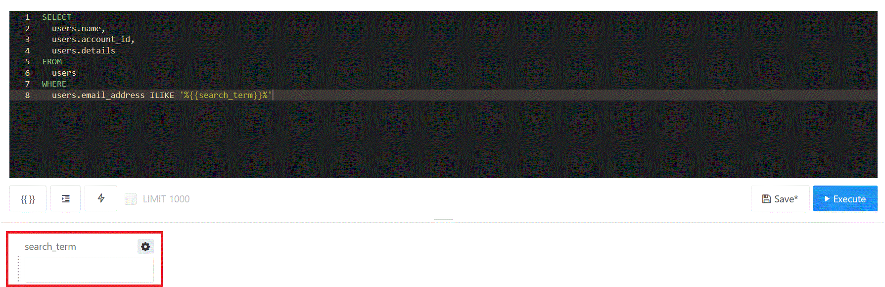
With parameters you can substitute values into your query at runtime without having to **Edit Source**. Any string between double curly braces `{{ }}` will be treated like a parameter. A widget will appear above the results pane so you change the parameter value.

<figure><img src="https://4269815422-files.gitbook.io/~/files/v0/b/gitbook-x-prod.appspot.com/o/spaces%2FGc9mnST31tkU3h2NNgSL%2Fuploads%2F9zIJTjk0Ap10ExO8essa%2Fsearch_term.gif?alt=media&amp;token=7303a1e2-a074-40ae-8313-5d4c4f75f34c" alt=""><figcaption></figcaption></figure>

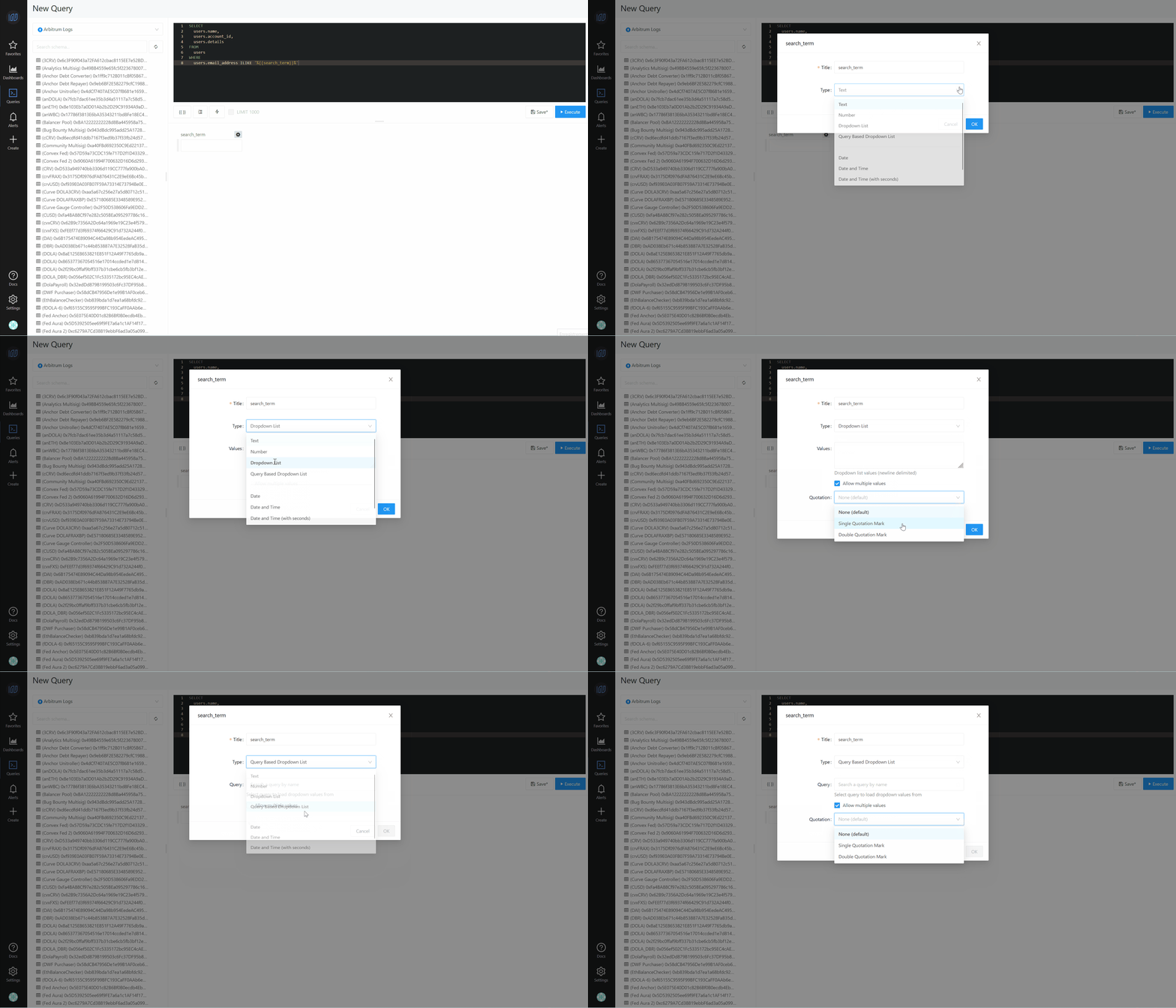
In editing mode, you can click the gear icon for each parameter widget to adjust its settings. The gear icons disappear when you click **Show Data Only** so that users who don’t own the query can’t change the parameter behavior.

<figure><img src="https://4269815422-files.gitbook.io/~/files/v0/b/gitbook-x-prod.appspot.com/o/spaces%2FGc9mnST31tkU3h2NNgSL%2Fuploads%2FmWVvuRAZCRUmOojG9I5n%2Fsearch_term_gear_icon.gif?alt=media&amp;token=27acba54-5d91-4b00-b459-ba94fa5361e4" alt=""><figcaption><p>search term gear icon</p></figcaption></figure>

### 1. Add A Parameter From The UI

You can insert a parameter into your query and immediately activate its settings pane by using the `Add Parameter` button or associated keyboard shortcut. The parameter will be inserted wherever the text caret appears in your query. If you find that you’ve inserted the parameter in the wrong part of the query, you can select the entire parameter (including the curly braces!) and cut/paste it wherever necessary.

{% hint style="info" %}
You can discover the key shortcut on your operating system by hovering your cursor above the `Add Parameter` button.
{% endhint %}

#### i. Parameter Settings

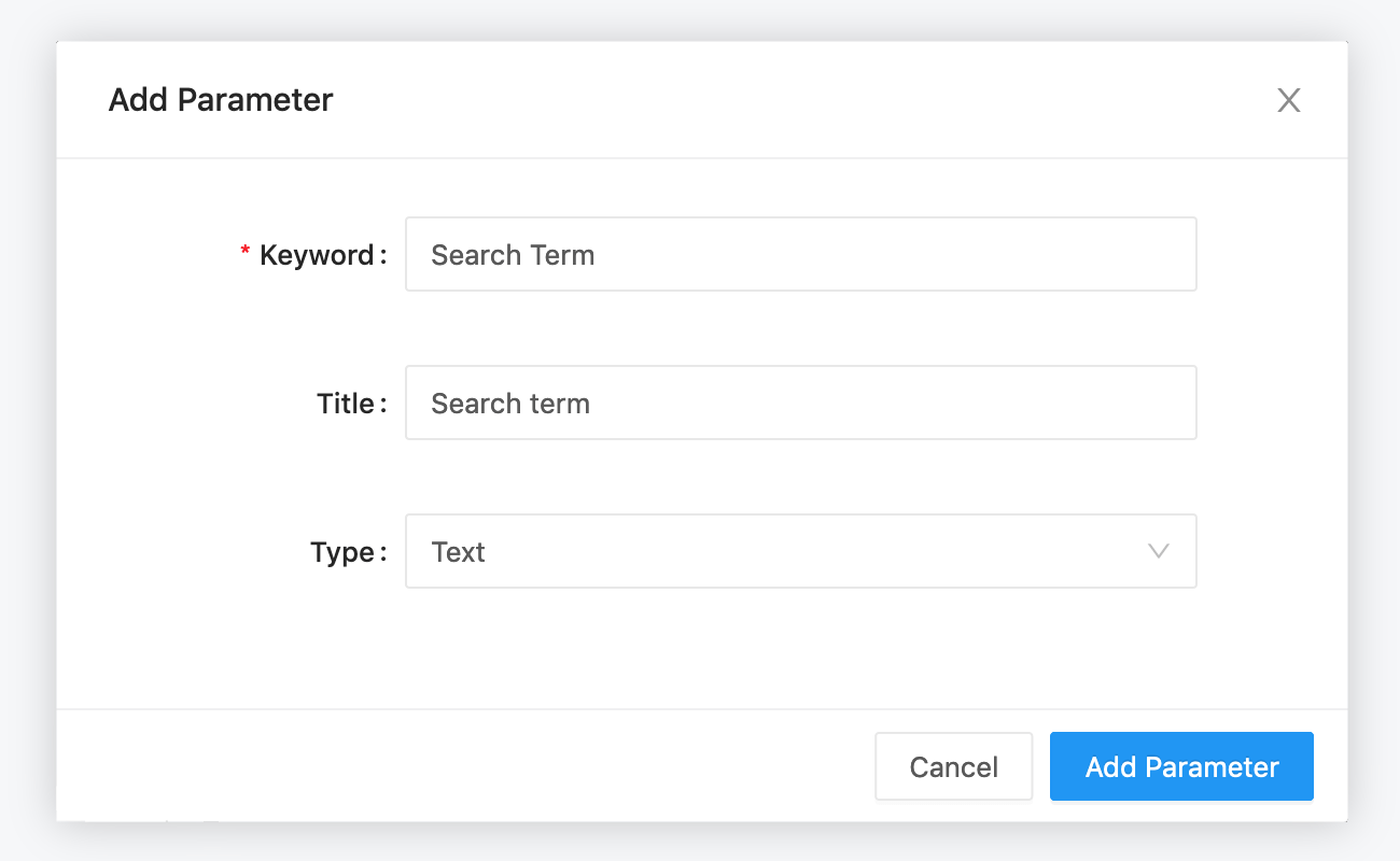
Click the gear icon beside each parameter widget to edit its settings:

* **Title** : by default the parameter title will be the same as the keyword in the query text. If you want to give it a friendlier name, you can change it here.
* **Type** : each parameter starts as a Text type. Supported types are Text, Number, Date, Date and Time, Date and Time (with Seconds), and Dropdown List.

<figure><img src="https://redash.io/assets/images/docs/gitbook/parameter-modal-v9.png" alt=""><figcaption></figcaption></figure>

{% hint style="danger" %}
For security reasons, user must have Full Access permission to the data source to use Text-type Query Parameters. Other types such as Date, Date Range, Number or Dropdown list are available to all users.
{% endhint %}

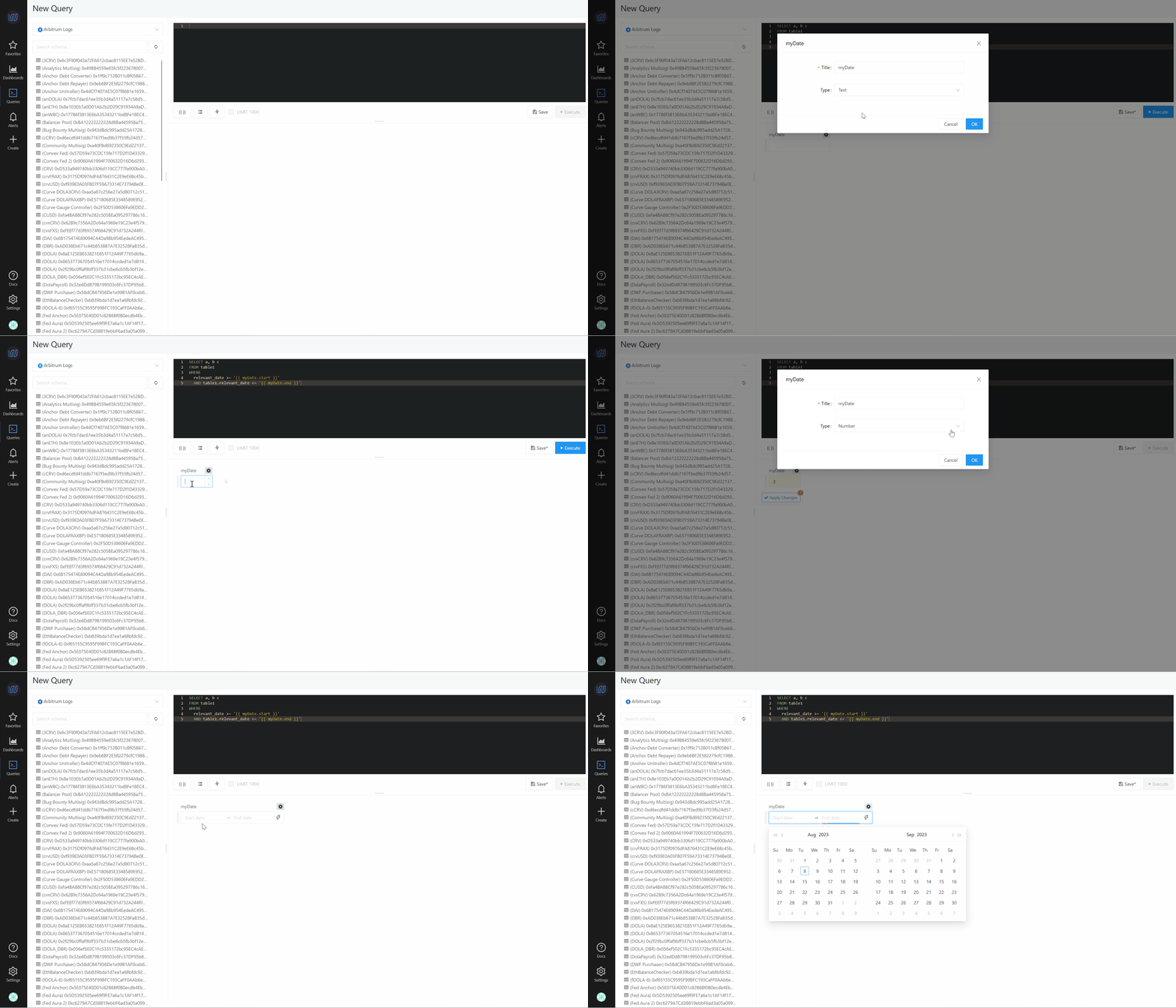
#### ii. Date and Date-Range Parameters

Date Parameters use a familiar calendar picking interface and can default to the current date and time. You can chose from three levels of precision: Date, Date and Time, and Date and Time with seconds.

Date Range Parameters insert two markers called `.start` and `.end` which signify the beginning and end of your chosen date range.

```
SELECT a, b c
FROM table1
WHERE
  relevant_date >= '{{ myDate.start }}'
  AND table1.relevant_date <= '{{ myDate.end }}'
```

{% hint style="info" %}
Date parameters are passed as strings to your database. So you should wrap them in single quotes (') or whatever your database uses to declare strings. Although they behave like Text parameters Dates are still safe for use in embeds and share dashboards.
{% endhint %}

Date Range parameters use a combined widget to simplify range selection.

<figure><img src="https://4269815422-files.gitbook.io/~/files/v0/b/gitbook-x-prod.appspot.com/o/spaces%2FGc9mnST31tkU3h2NNgSL%2Fuploads%2FYMc4ExBWNE0rWWhcPWan%2FDate-Range_Parameters.gif?alt=media&amp;token=977e68a6-21bb-4c50-8b91-b5041d61e841" alt=""><figcaption></figcaption></figure>

* Quick Date and Date-Range Options

When you add a Date or Date Range parameter to your query, the selection widget shows a blue lightning bolt glyph. Click the glyph to see dynamic values like “Today” or “Yesterday”.

There are dynamic date range options too. The complete list of dynamic date-ranges is:

* This week
* This month
* This year
* Last week
* Last month
* Last year
* Last 7 days
* Last 14 days
* Last 30 days
* Last 60 days
* Last 90 days
* Last 12 months

{% hint style="warning" %}
Because dynamic dates and date ranges are calculated in the front-end, they aren’t compatible with Scheduled Queries.
{% endhint %}

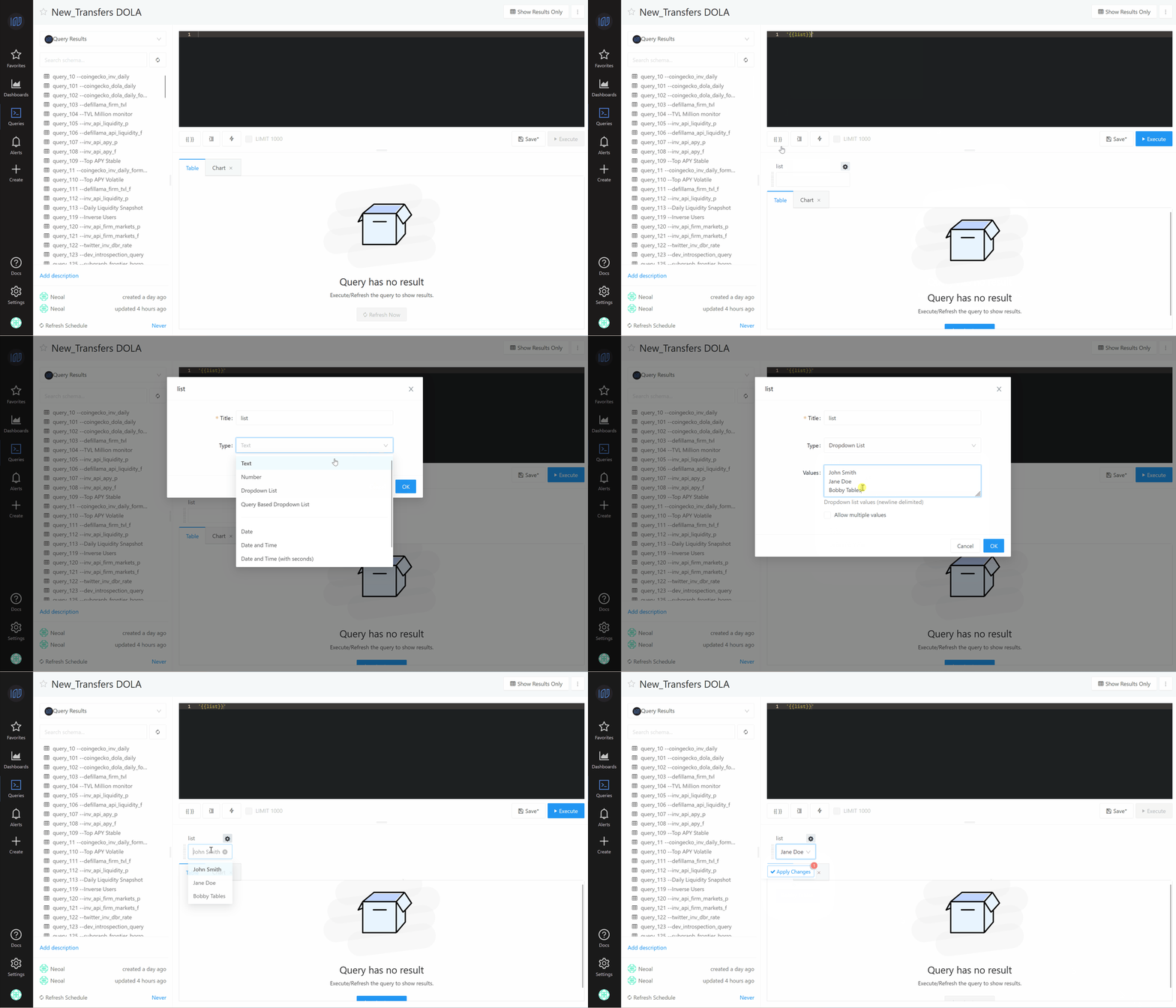
#### iii. Dropdown Lists

If you want to restrict the scope of possible parameter values when running a query, you can use the application’s `Dropdown List` parameter type. When selected from the parameter settings panel, a text box appears where you can enter your allowed values, each one separated by a new line. Dropdown lists are `Text` parameters under the hood, so if you want to use dates/datetimes in your dropdown, you should enter them in the format your data source requires.

<figure><img src="https://4269815422-files.gitbook.io/~/files/v0/b/gitbook-x-prod.appspot.com/o/spaces%2FGc9mnST31tkU3h2NNgSL%2Fuploads%2Ffwx2IotHiILDxmaK1RVD%2FDropdown%20Lists.gif?alt=media&amp;token=e01f7e9b-afa3-4544-b4fe-bcd165f4d0da" alt=""><figcaption></figcaption></figure>

* Query Based Dropdown List

Dropdown lists can also be tied to the results of an existing query. Just click `Query Based Dropdown List` under **Type** in the settings panel. Search for your target query in the **Query to load dropdown values from** bar. Performance will degrade if your target query returns a large number of records.

If your target query returns more than one column, the application uses the *first* one. If your target query returns `name` and `value` columns, the application populates the parameter selection widget with the `name` column but executes the query with the associated `value`.

For example, suppose this query:

```
SELECT user_uuid as ‘value’, username as ‘name’
FROM users
```

returned this data:

| value | name         |
| ----- | ------------ |
| 1001  | John Smith   |
| 1002  | Jane Doe     |
| 1003  | Bobby Tables |

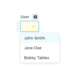
The application’s dropdown list widget would look like this:

<figure><img src="https://redash.io/assets/images/docs/gitbook/dropdown-list-name-value.png" alt=""><figcaption></figcaption></figure>

But when the application executes the query, the value passed to the database would be 1001, 1002 or 1003.

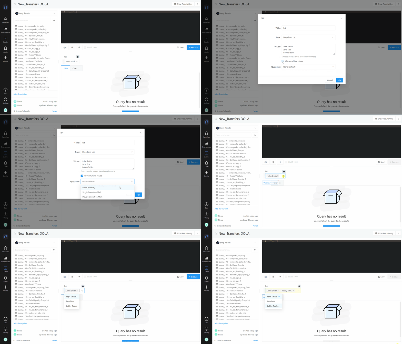
* Serialized Multi-Select

Dropdown lists can also be serialized to allow for multi-select. Just toggle the **Allow multiple values** option and choose whether or not to wrap the parameters with single quotes or double-quotes.

<figure><img src="https://4269815422-files.gitbook.io/~/files/v0/b/gitbook-x-prod.appspot.com/o/spaces%2FGc9mnST31tkU3h2NNgSL%2Fuploads%2FDINLdiz4tAJaOz0W5s0r%2FDropdown_list_multi.gif?alt=media&amp;token=2d4a139c-353c-4eda-98b6-accc2acc3c62" alt=""><figcaption></figcaption></figure>

In your query, change your `WHERE` clause to use the `IN` keyword.

```
SELECT ...
FROM   ...
WHERE field IN ( {{ Multi Select Parameter }} )
```

The parameter multi-selection widget let you pass extra values to the database.

#### iv. FAQ

**Can I reuse the same parameter multiple times in a single query?**

Sure! Just use the same identifier in the curly brackets. In this example:

```sql
SELECT {{org_id}}, count(0)
FROM queries
WHERE org_id = {{org_id}}
```

We use the `{{org_id}}` parameter twice.

**Can I use multiple parameters in a single query?**

Of course, just use a unique name for each one. In this example:

```sql
SELECT count(0)
FROM queries
WHERE org_id = {{org_id}} AND created_at > '{{start_date}}'
```

We use two parameters: `{{org_id}}` and `{{start_date}}`.

**Can I use parameters in embedded visualizations and shared dashboards?**

Yes, with one exception. If a query uses a Text type parameter it cannot be embedded because Text parameters are not safe from SQL injection. All other types of query parameters can be used safely in embedded visualizations and dashboards.

| Parameter Type                | Safe for Embedding? |
| ----------------------------- | ------------------- |
| Text                          | No                  |
| Number                        | Yes                 |
| Dropdown List                 | Yes                 |
| Query Based Dropdown List     | Yes                 |
| Date                          | Yes                 |
| Date and Time                 | Yes                 |
| Date and Time w/Seconds       | Yes                 |
| Date Range                    | Yes                 |
| Date and Time Range           | Yes                 |
| Date and Time Range w/Seconds | Yes                 |

**Can I change parameter values via the URL?**

Yes. Each parameter appears in the URL query string preceded by `p_`. A query with id `1234` and the following query text:

```
SELECT * FROM table WHERE field = {{param}}
```

Would have link a like so: `https://app.redash.io/<slug>/queries/1234?p_param=100`

This is useful for linking between queries and dashboards.

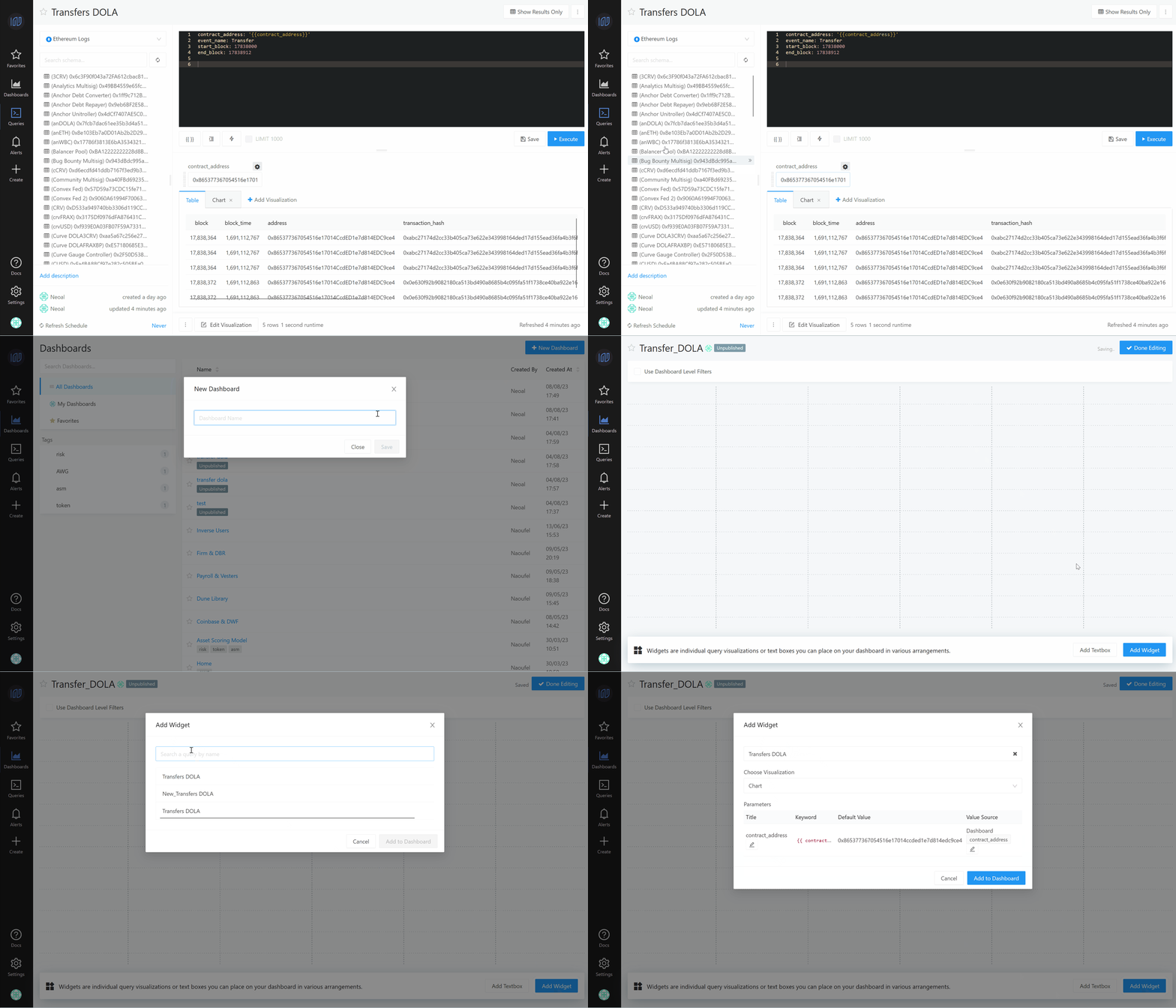
### 2. Parameter Mapping on Dashboards

Query Parameters can also be powerfully controlled within dashboards. You can link together parameters on different widgets, set static parameter values, or choose values individually for each widget.

You select your desired parameter mapping when adding dashboard widgets that depend on a parameter value. Each parameter in the underlying query will appear in the **Parameters** list.

<figure><img src="https://4269815422-files.gitbook.io/~/files/v0/b/gitbook-x-prod.appspot.com/o/spaces%2FGc9mnST31tkU3h2NNgSL%2Fuploads%2FHB03JUQ4cdWTZEdBBBCv%2FParameter%20Mapping%20on%20Dashboards.gif?alt=media&amp;token=8670cb76-1291-4b7c-a0f0-f2c96ee31844" alt=""><figcaption></figcaption></figure>

{% hint style="info" %}
You can also access the parameter mapping interface by clicking the vertical ellipsis (⋮) on the top right of a dashboard widget then clicking **Edit Parameters**.
{% endhint %}

* **Title** is the display name for your parameter and will appear beside the value selector on your dashboard. It defaults to the parameter keyword (see next bullet). Edit it by clicking the pencil glyph. Note that a titles are not displayed for static dashboard parameters because the value selector is hidden. If you select `Static value` as your Value Source then the Title field will be grayed out.
* **Keyword** is the string literal for this parameter in the underlying query. This is useful for debugging if your dashboard does not return expected results.
* **Default Value** is what the application will use if no other value is specified. To change this from the query screen, execute the query with your desired parameter value and click the **Save** button.
* **Value Source** is where you choose your preferred mapping. Click the pencil glyph to open the mapper settings.

#### i. Value Source Options

* **New dashboard parameter:** Dashboard parameters allow you to set a parameter value in one place on your dashboard and map it to multiple visualizations. Use this option to create a new dashboard-level parameter.
* **Existing dashboard parameter:** If you have already set up a dashboard-level parameter, use this option to map it to a specific query parameter. You will need to specify which pre-existing dashboard parameter will be mapped.
* **Widget parameter:** This option will display a value selector inside your dashboard widget. This is useful for one-off parameters that are not shared between widgets.
* **Static value:** Selecting this option will let you choose a static value for this widget, regardless of the values used on other widgets. Statically mapped parameter values do not display a value selector anywhere on the dashboard which is more compact. This lets you take advantage of the flexibility of Query Parameters without cluttering the user interface on a dashboard when certain parameters are not expected to change frequently.

#### &#x20;<a href="#faq" id="faq"></a>


# How to Schedule a Query

You can use scheduled query executions to keep your dashboards updated or to power routine Alerts. By default, your queries will not have a schedule. But this is easy to adjust. In the bottom left corner of the query editor you’ll see the schedule area.

Clicking **Never** will open a picker with allowed schedule intervals.

<figure><img src="https://4269815422-files.gitbook.io/~/files/v0/b/gitbook-x-prod.appspot.com/o/spaces%2FGc9mnST31tkU3h2NNgSL%2Fuploads%2FqG6YZXzBBpbLAijmJ1eT%2FSchedule%20a%20Query.gif?alt=media&amp;token=c84c5c1e-c573-434e-8e4b-b2e7c56cab6f" alt=""><figcaption><p>schedule a query</p></figcaption></figure>

Your query will run automatically once a schedule is set.

When you schedule queries to run at a certain time-of-day, the application converts your selection to UTC using your computer’s local timezone. That means if you want a query to run at a certain time in UTC, you need to adjust the picker by your local offset.

For example, if you want a query to execute at `00:00` UTC each day but your current timezone is CDT (UTC-5), you should enter `19:00` into the scheduler. The UTC value is displayed to the right of your selection to help confirm your math.

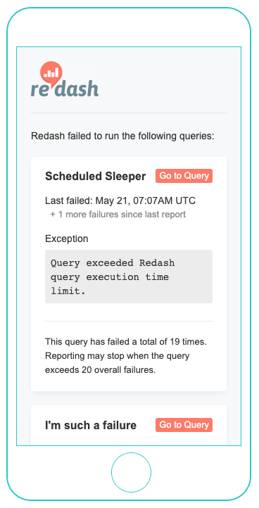
### Scheduled Query Failure Reports <a href="#scheduled-query-failure-reports" id="scheduled-query-failure-reports"></a>

The application has the ability to email query owners once per hour if one or more queries failed. These emails continue until there are no more failures. Failure report emails run on an independent process from the actual query schedules. It may take up to an hour after a failed query execution before the application sends the failure report.

You can toggle failure reports from your organizations settings. Under **Feature Flags** check **Email query owners when scheduled queries fail**.

<figure><img src="https://redash.io/assets/images/docs/gitbook/failure-report.png" alt=""><figcaption></figcaption></figure>


# Favorites & Tagging

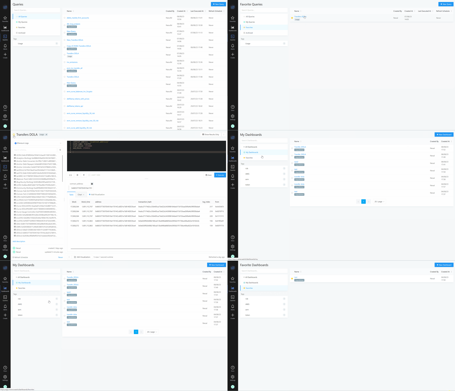
Users will write a lot of queries and dashboards! Favorites and Tagging are here to make finding them easy as your collection of queries and dashboards grows from a few hundred to a few thousand.

<figure><img src="https://4269815422-files.gitbook.io/~/files/v0/b/gitbook-x-prod.appspot.com/o/spaces%2FGc9mnST31tkU3h2NNgSL%2Fuploads%2F1HRERFzQ8sTmz1na1TuD%2Ffavorite%20%26%20tag.gif?alt=media&amp;token=367630a1-258e-45a1-bd35-16722d704055" alt=""><figcaption><p>Favorites &#x26; Tagging</p></figcaption></figure>

### 1. Favorites

You can favorite a dashboard or query by clicking the star to the left of its title anywhere in the application. The star will turn yellow to indicate success. Your favorites are displayed at several places in the application. They appear on the homepage, in the navbar dropdown menus and as filters in the query or dashboard list views.

<figure><img src="https://4269815422-files.gitbook.io/~/files/v0/b/gitbook-x-prod.appspot.com/o/spaces%2FGc9mnST31tkU3h2NNgSL%2Fuploads%2Fr5TwnAWRHPUTTv1KCrMm%2Ffavorites.gif?alt=media&amp;token=ef44248f-ce0b-43ed-a951-a1fe23ef5440" alt=""><figcaption><p>Favorites</p></figcaption></figure>

### 2. Tagging

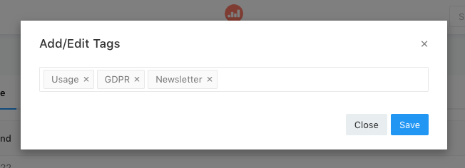
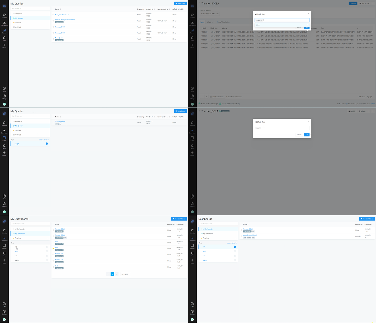
You can tag queries and queries by subject matter, location, user or any parameter that is meaningful to your organization. Tags are added from the query editor or the dashboard editor. Hover your mouse on the query or dashboard title and an `+Add Tag` button will appear. In the modal that appears you can select as many tags as you need. The modal will suggest previously-used tags as you type. Hit `Save` when you’re finished or `Esc` to abort tagging.

{% hint style="info" %}
It’s important to have predictable taxonomy for your tags. Consistency in this area makes using the application an even nicer experience and helps bring new users onboard. So we recommend that your team have an internal discussion about the tag hierarchy that will be most beneficial to your organization.
{% endhint %}

<figure><img src="https://redash.io/assets/images/docs/gitbook/tagging-example.png" alt=""><figcaption><p>Tagging</p></figcaption></figure>

Your tags will appear on the Dashboard and Query list views on the righthand side. You can filter the by tag by cliking on the desire tag on the tag section. Click a second time to remove the filter. `Shift + Click` to select multiple filters

<figure><img src="https://4269815422-files.gitbook.io/~/files/v0/b/gitbook-x-prod.appspot.com/o/spaces%2FGc9mnST31tkU3h2NNgSL%2Fuploads%2F1IeGfed1SsvsCtOecEFE%2Ftagging.gif?alt=media&amp;token=b554d0f7-055c-44da-a477-924f84364a85" alt=""><figcaption><p>tagging</p></figcaption></figure>

### &#x20;<a href="#favorites" id="favorites"></a>


# Query Filters

Query Filters let you interactively reduce the amount of data shown in your visualizations, similar to Query Parameters but with a few key differences. Query Filters limit data **after** it has been loaded into your browser. This makes them ideal for smaller datasets and environments where query executions are time-consuming, rate-limited, or costly.

### 1. Usage

Unlike Query Parameters there isn’t a button to add a filter. Instead, if you want to focus on a specific value, just alias your column to `<columnName>::filter`. Here’s an example:

```sql
SELECT action AS "action::filter", COUNT(0) AS "actions count"
FROM events
GROUP BY action
```

{% hint style="info" %}
Note that you can use<mark style="background-color:blue;">`__filter`</mark> or <mark style="background-color:blue;">`__multiFilter`</mark>, (double underscore instead of double quotes) if your database doesn’t support :: in column names (such as BigQuery).
{% endhint %}

![](https://redash.io/assets/images/docs/gitbook/filter_example_action_create.png)

If you need a multi-select filter then alias your column to `<columnName>::multi-filter`.

```
SELECT action AS "action::multi-filter", COUNT (0) AS "actions count"
FROM events
GROUP BY action
```

![](https://redash.io/assets/images/docs/gitbook/multifilter_example.png)

You can use Query Filters on dashboards too. By default, the filter widget will appear beside each visualization where the filter has been added to the query. If you’d like to link together the filter widgets into a dashboard-level Query Filter see [these instructions](https://redash.io/help/user-guide/dashboards/dashboard-editing).

### 2. Limitations

Query Filters aren’t suitable for especially large data sets or query results with hundreds or thousands of distinct field values. Depending on your computer and browser configuration, excessive data can deteriorate the user experience.


# How To Download / Export Query Results

### 1. How to download a query result

Visit any query page and click the vertical ellipsis (`⋮`) button beneath the results pane. Then choose to download a CSV, TSV, or Excel file. This action downloads the current query result.

<figure><img src="https://4269815422-files.gitbook.io/~/files/v0/b/gitbook-x-prod.appspot.com/o/spaces%2FGc9mnST31tkU3h2NNgSL%2Fuploads%2FVuVre5c7ZeTZ1z1PPWGk%2FDownload_query.gif?alt=media&amp;token=31437bf7-c696-4d5b-9734-85cf69c1f98f" alt=""><figcaption><p>download query results</p></figcaption></figure>

### 2. How to get latest results via the API

Visit any query page and click the horizontal ellipsis (`…`) above the query editor. Then choose **Show API Key**. The links in the modal that appears always point to the latest query result. You can choose between CSV and JSON formats to be returned by the API call.

{% hint style="info" %}
It’s not shown in the interface, but you can also get the Excel format by changing the file type suffix from `json`/`csv` to `xlsx`.
{% endhint %}

<figure><img src="https://4269815422-files.gitbook.io/~/files/v0/b/gitbook-x-prod.appspot.com/o/spaces%2FGc9mnST31tkU3h2NNgSL%2Fuploads%2F0x6lJDSi146p4RXALHig%2Fshow_api.gif?alt=media&amp;token=d86a3c8c-be02-4a21-ba8b-dd01c1e2e7b6" alt=""><figcaption><p>show API</p></figcaption></figure>

{% hint style="warning" %}
The latest results API is not supported for queries that use parameters.
{% endhint %}


# Query Snippets

### 1. Create A Query Snippet

Copy and Paste are a big part of composing database queries. Because it’s much easier to duplicate prior work than to write it from scratch. This is particularly true for common `JOIN` statements or complex `CASE` expressions. As your list of queries in the application grows, however, it can be difficult to remember which queries contain the statement you need right now. Enter Query Snippets.

Query Snippets are segments of queries that your whole team can share and trigger via auto complete. You create them at `Settings` -> `Query Snippets`.

Here’s an example for a simple snippet:

```
JOIN organizations org ON org.id = ${1:table}.org_id
```

<figure><img src="https://4269815422-files.gitbook.io/~/files/v0/b/gitbook-x-prod.appspot.com/o/spaces%2FGc9mnST31tkU3h2NNgSL%2Fuploads%2FNzvFrjrkfeF8tMWARZ3y%2Fcreate_snippets.gif?alt=media&amp;token=fdacf179-e21c-4b56-9a50-cc587db48ce2" alt=""><figcaption><p>create a query snippets</p></figcaption></figure>

### 2. Insert A Query Snippet

If you have Live Auto Complete enabled, you can invoke your snippet from the Query Editor by typing the trigger word you defined in the Query Snippet editor. Auto Complete will suggest it like any other keyword in your database.

Here are some other ideas for snippets:

* Frequent `JOIN` statements
* Complicated clauses like `WITH` or `CASE`.
* [Conditional Formatting](https://discuss.redash.io/t/conditional-formatting-general-text-formatting/1706/1)

When the application renders the snippet, the dollar sign `$` and curly braces `{}` will be stripped away and the word `table` will be highlighted for the user to replace.

<figure><img src="https://4269815422-files.gitbook.io/~/files/v0/b/gitbook-x-prod.appspot.com/o/spaces%2FGc9mnST31tkU3h2NNgSL%2Fuploads%2FjyaykK86F95LUeFZGUt0%2Finsert_snippets.gif?alt=media&amp;token=95e9bc65-0c9e-423b-b72d-9c9bd9d126e7" alt=""><figcaption><p>insert a query snippet</p></figcaption></figure>

When the application renders the snippet, the dollar sign `$` and curly braces `{}` will be stripped away and the word `table` will be highlighted for the user to replace.

<figure><img src="https://4269815422-files.gitbook.io/~/files/v0/b/gitbook-x-prod.appspot.com/o/spaces%2FGc9mnST31tkU3h2NNgSL%2Fuploads%2FnS5XVzN4GGaN3NuygQQu%2Fcreate_snippets.gif?alt=media&amp;token=94c7a8fa-5442-4110-853d-0c6f1edfe73d" alt=""><figcaption><p>create query snippets</p></figcaption></figure>

### 3. Insertion Points

In the example above, `${1:table}` is an insertion point with placeholder text.&#x20;

In the example above, `${1:table}` is an insertion point with placeholder text.

{% hint style="info" %}
You can use the placeholder text as a desirable default value for the user to override at runtime.
{% endhint %}

You designate insertion points by wrapping an integer tab order with a single dollar sign and curly braces `${}`. A text placeholder preceded by a colon `:` is optional but useful for users unfamiliar with your snippet.

When the application renders this snippet:

```
AND (invoices.complete IS NULL OR invoices.complete <> '${2}')
AND (invoices.canceled IS NULL OR invoices.canceled <> '${1}')
AND (invoices.modified IS NULL OR invoices.modified_date <> '${0: this_date}')
```

The text insertion carat will jump to the second line between the quote marks `''`. When the user presses `Tab` the carat will jump *backwards* onto the first line. When the user presses `Tab` again, the carat will jump to the third line and `this_date` will be highlighted to prompt the user for the desired value.

<figure><img src="https://4269815422-files.gitbook.io/~/files/v0/b/gitbook-x-prod.appspot.com/o/spaces%2FGc9mnST31tkU3h2NNgSL%2Fuploads%2FXQHISjsgaFKHedpEQLCR%2Fsnippets_insertion_points.gif?alt=media&amp;token=ab150117-aa45-4f66-aff1-ca42019e4bec" alt=""><figcaption><p>query snippet insertion points</p></figcaption></figure>

{% hint style="info" %}
An insertion point of zero `${0}` is always the *last* point in the tab order.
{% endhint %}

{% hint style="warning" %}
If Live Auto Complete is disabled, you can still invoke Query Snippets by pressing `CTRL + Space` and typing the trigger word for your Query Snippet. This can be necessary if your schema exceeds 5000 tokens.
{% endhint %}


# Visualizations


# Cohort Visualizations

## Cohorts Introduction <a href="#cohorts-introduction" id="cohorts-introduction"></a>

A cohort analysis examines the outcomes of predetermined groups, called cohorts, as they progress through a set of stages. The signature characteristic of a cohort chart is its comparison of the change in a variable across two different time series. For example, a common cohort definition is users by sign-up period and their usage pattern by day. Other examples include:

* Monthly hard drive failure statistics by month
* Weekly supplier delivery performance by week
* Monthly average class GPA’s by month

While there are many ways to define the stages of a Cohort analysis, the application supports Cohorts visualizations with daily, weekly, or monthly stages. Also, the application's cohort charts compare a cohort’s measurements in a given period against that group’s initial population size.

#### i. Data Format

The application expects your input samples to take the following format:

* **Cohort Date** is the date that uniquely identifies a cohort. Suppose you’re visualizing monthly user activity by sign-up date, your cohort date for all users that signed-up in January 2018 would be January 1st, 2018. The cohort date for any user that signed-up in February would be February 1st, 2018.
* **Period** is a count of how many periods transpired since the cohort date as of this sample. If you are grouping users by sign-up month, then your period will be the count of months since these users signed up. In the above example, a measurement of activity in July for users that signed up in January would yield a period value of 7 because seven periods have transpired between January and July.
* **Count Satisfying Target** is your actual measurement of this cohort’s performance in the given period. In the above example, if thirty users who signed up in January showed activity in July then the Count Satisfying Target would be 30.
* **Total Cohort Size** is the denominator that the application will use to calculate the percentage of a cohort’s target satisfaction for a given period. Continuing the example above, if seventy-two users signed up in January then the Total Cohort Size would be 72. When the visualization is rendered, the application would display the value as 41.67% (32 ÷ 72).

###


# Visualizations How-To

### 1. Create a New Visualization <a href="#create-a-new-visualization" id="create-a-new-visualization"></a>

Once your query has finished running for the first time, you can add a visualization by clicking the “New Visualization” button above the results table.

<figure><img src="https://4269815422-files.gitbook.io/~/files/v0/b/gitbook-x-prod.appspot.com/o/spaces%2FGc9mnST31tkU3h2NNgSL%2Fuploads%2FoCGlVssVsXmhg15bghrx%2Fcreate_new_visualization.gif?alt=media&amp;token=36a2206c-2df5-4b40-9c1e-4fe36814619e" alt=""><figcaption><p>create a new visualization</p></figcaption></figure>

### 2. Edit A Visualization

You can modify the settings of an existing visualization from the query editor screen. Click the visualization on the tab bar and you’ll see an `Edit Visualization` option beneath each visualization. Clicking it will open the current settings for that visualization (type, X axis, Y axis, groupings etc.). Hit “Save” to apply your changes or “Cancel” to leave no trace.

<figure><img src="https://4269815422-files.gitbook.io/~/files/v0/b/gitbook-x-prod.appspot.com/o/spaces%2FGc9mnST31tkU3h2NNgSL%2Fuploads%2FyntGYMLTPri2xfoEyOgy%2FEdit_A_Visualization.gif?alt=media&amp;token=5cacd680-104e-41f8-a3ed-5b580bd03f5f" alt=""><figcaption><p>edit a visualization</p></figcaption></figure>

### 3. Embedding Visualizations

It’s easy to embed visualizations. Just click the ellipsis button beneath any visualization to show further options and select `Embed Elsewhere`.

This will pop up the `<iframe>` code you can drop into your HTML pages.

<figure><img src="https://4269815422-files.gitbook.io/~/files/v0/b/gitbook-x-prod.appspot.com/o/spaces%2FGc9mnST31tkU3h2NNgSL%2Fuploads%2FLvfqr6g032ToLF5mDyOi%2FEmbedding_Visualizations.gif?alt=media&amp;token=48937fbc-35b2-4733-b069-a79aeeb6b9da" alt=""><figcaption><p>embedding visualization</p></figcaption></figure>

{% hint style="warning" %}
Queries with text-type parameters do not support embeds
{% endhint %}

**PNG image Embeds**

For SaaS customers, there is also a hardlink to a PNG of your visualization hosted through `snap.redash.io`. The PNG embed is especially useful in contexts where iframes won’t work (like GitHub issues). If you need the visualization PNG to include a `Cache-Control: no-cache` header, just tack the Query String variable `?no-cache` to the end of your PNG embed link.

**Query String Variables for Embeds**

You can append query string variables to your embed URLs:

* `?hide_parameters` hides any parameter selection widgets
* `?hide_timestamp` hides the timestamp

**Downloading A Visualization as an Image File**

For chart visualizations, you can also download a local image file. Just hover your mouse near the top right area of the visualization and click the camera icon that appears. A PNG will be downloaded to your device.

<figure><img src="https://4269815422-files.gitbook.io/~/files/v0/b/gitbook-x-prod.appspot.com/o/spaces%2FGc9mnST31tkU3h2NNgSL%2Fuploads%2FWUn2y9QtKos4u2ecK9pN%2FDownloading%20A%20Visualization%20as%20an%20Image%20File.gif?alt=media&amp;token=ca53bc55-0637-4043-bf07-51a00ddd4260" alt=""><figcaption><p>visualization png file</p></figcaption></figure>

***


# Chart Visualizations

The application bundles together charts that use X & Y axes into the **Chart** visualization type, which can take eight different forms. Because the forms are similar, you can often switch seamlessly between them to find the one that best conveys your meaning. In the animation below, all eight charts were built from the same SQL query result:

<figure><img src="https://4269815422-files.gitbook.io/~/files/v0/b/gitbook-x-prod.appspot.com/o/spaces%2FGc9mnST31tkU3h2NNgSL%2Fuploads%2FRTCNSg10mnfVeSaaBr8b%2Fvisualization_charts.gif?alt=media&amp;token=417def71-7497-4052-ba9c-27114ece6974" alt=""><figcaption><p>chart visualization type</p></figcaption></figure>

The charts in the above animation were all produced from the following tabular result:

<figure><img src="https://4269815422-files.gitbook.io/~/files/v0/b/gitbook-x-prod.appspot.com/o/spaces%2FGc9mnST31tkU3h2NNgSL%2Fuploads%2FYFtf61JcF5f63HvKDpC7%2Ftable_charts.gif?alt=media&amp;token=362d0bd6-c974-4474-9b18-b37c990e6d05" alt="" width="563"><figcaption></figcaption></figure>

### 1. Setup

Once you have run your query, you will receive your table. You can adjust the table's visualization as needed.

<figure><img src="https://4269815422-files.gitbook.io/~/files/v0/b/gitbook-x-prod.appspot.com/o/spaces%2FGc9mnST31tkU3h2NNgSL%2Fuploads%2FrMM7a9gSbbtaCUxNfGuX%2Ftable_visualization_settings.gif?alt=media&amp;token=912705d2-0fb7-43ad-abc7-04fddefd3de4" alt=""><figcaption><p>table visualization settings</p></figcaption></figure>

Then, you can add a visualization and modify the settings. Your query should return at least two columns: one column of values for the **X axis** and one column of values for the **Y Axis**. It can also return values for trace [grouping](https://redash.io/help/user-guide/visualizations/chart-visualizations#Grouping), displaying [error bars,](https://redash.io/help/user-guide/visualizations/chart-visualizations#Error-Bars) and bubble sizes.

Once your query returns the right columns, start by setting your X and Y axis values. The visualization preview updates instantly. You don’t need to save the visualization to see how a change affects its appearance. Tabs on the Visualization Settings screen give you fine-grained control over the rest of chart.

Use the **X Axis** and **Y Axis** tabs to modify the axis ranges and labels.

The **Series** tab is powerful. It lets you change your data aliases, z-index behavior, assign traces between the left- and right- Y axes. It also lets you combine different trace forms on one chart like in the chart below.

<figure><img src="https://4269815422-files.gitbook.io/~/files/v0/b/gitbook-x-prod.appspot.com/o/spaces%2FGc9mnST31tkU3h2NNgSL%2Fuploads%2FH7152COfqrwzaeW8GBRJ%2Fseries.gif?alt=media&amp;token=a3da69dc-c498-4542-b5e6-7d3212f76421" alt=""><figcaption></figcaption></figure>

**Colors** gives you a color picker for changing the appearance of the traces on your charts.

**Data Labels** controls what appears when you hover your mouse over a chart.

<figure><img src="https://4269815422-files.gitbook.io/~/files/v0/b/gitbook-x-prod.appspot.com/o/spaces%2FGc9mnST31tkU3h2NNgSL%2Fuploads%2Fsts7wR5Li4oXKNY3IIig%2Fvisualization_settings.gif?alt=media&amp;token=f433bd98-f64b-4b59-b0b5-32a53ffc80c5" alt=""><figcaption><p>visualizations settings</p></figcaption></figure>

### 2. Grouping

The **Group By** setting can generate multiple traces against the same X and Y axes. It does this by grouping records into distinct traces instead of drawing one line. Almost every time you see multiple colors of line or bar in a chart, it’s because the query results included a grouping column.

As shown in the below example, the grouping column is used to sort `(x,y)` pairs together.

![](https://redash.io/assets/images/docs/gitbook/group-by-ex.png)

Use of **Group By** is often easier than writing queries which return multiple Y columns for an X value. The following two data sets are identical.

![](https://redash.io/assets/images/docs/gitbook/grouped-vs-pivot.png)

{% hint style="info" %}
Use the **Group By** column for melted data sets. Use multiple Y-columns for pivoted data sets
{% endhint %}

### 3. Stacking

The application can “stack” your Y axis values on top of one another. The name name is borrowed from [Stacked Bar Charts](https://en.wikipedia.org/wiki/Bar_chart#Grouped_and_stacked), but it can be useful with area charts as well. The below image shows the same data, unstacked on the left and stacked on the right.

![](https://redash.io/assets/images/docs/gitbook/stacked_vs_not_stacked.png)

Notice how each Y axis value is displayed as the sum of itself and the Y values “beneath” it.

{% hint style="info" %}
Stacking and Grouping are related. You won’t stack data unless you have also grouped it.
{% endhint %}

You can use the **Series** tab of the Visualization Editor to control the order in which traces are stacked. You can also control it by adding an `ORDER BY` statement to your query. The stack follows the order in which your group names first appear in your query result. Stacking is only available for Line, Bar, and Area charts.

### 4. Error Bars

For certain chart forms, the application can draw error bars around your data points using values from your query result. A few things are always true of error bars:

1. Error bars are always symmetrical. The distance above and below a given `(x,y)` pair is always the same.
2. Errors are the same color as their target trace
3. Errors are shown for all traces or no traces. They cannot be configured to appear on some traces and not others.
4. The values in your errors column will be charted on the same axis as their associated trace. This means your error values must be absolute. You cannot, for example, have errors expressed in percentages for Y values expressed in hundreds.

![](https://redash.io/assets/images/docs/gitbook/area_grouped_stacked_errors.png)

Also keep in mind that errors are not aggregated when you stack records. An error bar will be shown for each trace. You can work around this by only providing non-zero error values for those records where the error should be displayed prominently. See in the above example that a flat error bar is shown at every trace point. But only the `Paid` trace error bars have any length.

### 5. Using Chart Forms

Each chart form is useful for certain kinds of presentation. You can mix and match multiple forms on the same chart as needed.

* **Line** charts are almost exclusively used to present change in one or more metrics over *time*.
* **Bar** charts can be used to present change in metrics over time or to show proportionality, like a pie chart. Bar charts can be combined with [Stacking](https://redash.io/help/user-guide/visualizations/chart-visualizations#Stacking) with great effect. Horizontal bar charts are also supported.
* **Area** charts are often used to show sales funnel changes through time. They are frequently combined with [Stacking](https://redash.io/help/user-guide/visualizations/chart-visualizations#Stacking) to grant a broader picture.
* **Pie** charts are designed to show proportionality between metrics. They are *not* meant for conveying time series data.
* **Scatter** charts excel at showing many groups of data points. Under the covers, Scatter plots are just like line plots, but without the connecting lines. A scatter graph is more precise but less useful for time series data.

{% hint style="info" %}
Scatter plots are necessary for visualizations where some groups appear just once. The line chart does not display singleton values because it can only show data where two or more points are present. One option is to force singletons into scatter form on the **Series** tab of the Visualization Editor while keeping other traces in line form.
{% endhint %}

* **Bubble** charts are scatter graphs where the size of each point marker reflects a relevant metric.
* **Heatmap** visualizations blend features of bar charts, stacking, and bubble charts. There are several built-in color schemes to pick from. Heatmaps cannot be grouped since the entire chart is technically one trace.
* **Box** plots can automatically show the distribution of data points across grouped categories. Horizontal box plots are also supported.

### 6. Common Mistakes

* Multiple Records per X-axis value

The application can make some crazy shapes if your query returns two or more rows with the same **X axis** value. This often happens in SQL if you unintentionally `JOIN` a table with a one-to-many relationship.

![](https://redash.io/assets/images/docs/gitbook/error_double_entries.png)

In this example a vertical line is drawn because there are two records for 1 January. You can resolve this by filtering out the doubled entries on the **X axis**. Or revise the query to include [grouping](https://redash.io/help/user-guide/visualizations/chart-visualizations#Grouping) field, as shown below.

![](https://redash.io/assets/images/docs/gitbook/error_double_entries__solved.png)

### &#x20;<a href="#unordered-x-axis-records" id="unordered-x-axis-records"></a>

* Unordered X-axis records

The application is smart enough to figure out most common **X axis** scales: timestamps, linear, and logarithms. But if it can’t parse your X column into an ordered series, it falls back to treating each X value as a “category”. This can have mixed results:

![](https://redash.io/assets/images/docs/gitbook/charted_redash_logo__broken.png)

If you see shapes you don’t expect you can check whether your X axis has been sorted on the **X Axis** tab of the Visualization Editor. Just toggle the *Sort Values* option. If *Sort Values* is disabled then the application retains the ordering of the source query.

![](https://redash.io/assets/images/docs/gitbook/charted_redash_logo__working.png)

These two charts come from the same base data. The only difference is whether or not the application sorted the X axis values.

### &#x20;


# Formatting Numbers in Visualizations

In several visualizations you can control how the numbers are formatted in the Visualization Editor / Data Labels . You control the format by supplying a format string. Below you can find examples for the various format options.

### 1. Numbers

| Number     | Format     | Output        |
| ---------- | ---------- | ------------- |
| 10000      | 0,0.0000   | 10,000.0000   |
| 10000.23   | 0,0        | 10,000        |
| 10000.23   | +0,0       | +10,000       |
| -10000     | 0,0.0      | -10,000.0     |
| 10000.1234 | 0.000      | 10000.123     |
| 100.1234   | 00000      | 00100         |
| 1000.1234  | 000000,0   | 001,000       |
| 10         | 000.00     | 010.00        |
| 10000.1234 | 0\[.]00000 | 10000.12340   |
| -10000     | (0,0.0000) | (10,000.0000) |
| -0.23      | .00        | -.23          |
| -0.23      | (.00)      | (.23)         |
| 0.23       | 0.00000    | 0.23000       |
| 0.23       | 0.0\[0000] | 0.23          |
| 1230974    | 0.0a       | 1.2m          |
| 1460       | 0 a        | 1 k           |
| -104000    | 0a         | -104k         |
| 1          | 0o         | 1st           |
| 100        | 0o         | 100th         |

### &#x20;<a href="#currency" id="currency"></a>

### 2. Currency

| Number    | Format      | Output     |
| --------- | ----------- | ---------- |
| 1000.234  | $0,0.00     | $1,000.23  |
| 1000.2    | 0,0\[.]00 $ | 1,000.20 $ |
| 1001      | $ 0,0\[.]00 | $ 1,001    |
| -1000.234 | ($0,0)      | ($1,000)   |
| -1000.234 | $0.00       | -$1000.23  |
| 1230974   | ($ 0.00 a)  | $ 1.23 m   |

### 3. Bytes

| Number        | Format   | Output    |
| ------------- | -------- | --------- |
| 100           | 0b       | 100B      |
| 1024          | 0b       | 1KB       |
| 2048          | 0 ib     | 2 KiB     |
| 3072          | 0.0 b    | 3.1 KB    |
| 7884486213    | 0.00b    | 7.88GB    |
| 3467479682787 | 0.000 ib | 3.154 TiB |

### 4. Percentages

| Number     | Format    | Output   |
| ---------- | --------- | -------- |
| 100        | 0%        | 100%     |
| 97.4878234 | 0.000%    | 97.488%  |
| -4.3       | 0 %       | -4 %     |
| 65.43      | (0.000 %) | 65.430 % |

### 5. Exponential

| Number       | Format   | Output   |
| ------------ | -------- | -------- |
| 1123456789   | 0,0e+0   | 1e+9     |
| 12398734.202 | 0.00e+0  | 1.24e+7  |
| 0.000123987  | 0.000e+0 | 1.240e-4 |


# How to Make a Pivot Table

### Intro

The application’s pivot table visualization can aggregate records from a query result into a new tabular display. It’s similar to `PIVOT` or `GROUP BY` statements in SQL. But the visualization is configured with drag-and-drop fields instead of SQL code.

## Step 1: Write a query <a href="#step-1-write-a-query" id="step-1-write-a-query"></a>

It should return at least three columns. The source query for a pivot table is usually non-aggregated or "melted", and not necessarily sorted the way we want.&#x20;

<figure><img src="https://4269815422-files.gitbook.io/~/files/v0/b/gitbook-x-prod.appspot.com/o/spaces%2FGc9mnST31tkU3h2NNgSL%2Fuploads%2Fn0TWvGV7VCTWNjuidufZ%2Fpivot_table_write_a_query.gif?alt=media&amp;token=d58d3164-e048-48f9-bceb-f764ba2e3cdf" alt=""><figcaption></figcaption></figure>

We will use the pivot table to do this without SQL.

## Step 2: Add a **Pivot Table** visualization <a href="#step-2-add-a-pivot-table-visualization" id="step-2-add-a-pivot-table-visualization"></a>

Click **Add Visualization** and choose **Pivot Table** as the visualization type. The visualization preview on the right will update to show a pivot table.

All the field aliases from your query result become available at the top of the pivot control surface. You can drag these to the *row* side or the *column* side. You can also nest them.

Here is a simple example using the data from the above query:

<figure><img src="https://4269815422-files.gitbook.io/~/files/v0/b/gitbook-x-prod.appspot.com/o/spaces%2FGc9mnST31tkU3h2NNgSL%2Fuploads%2FfhOL7pwdTm56iq0y4Lt4%2Fpivot_table_bis.gif?alt=media&amp;token=c47d1155-3a56-4444-bf22-1c88b45d5981" alt=""><figcaption><p>pivot table</p></figcaption></figure>

{% hint style="warning" %}
Pivot table performance can degrade if your query result is too big. The exact size threshold will depend on the computer and browser from which you access the application. But in general, performance is best below 50,000 *fields*. That could mean 10,000 records with 5 fields each. Or 1,000 records with 50 fields each.
{% endhint %}


# Funnel Visualizations

The Funnel Visualization is available on the **Visualization Type** menu. It’s easy to make because it needs only two fields from your query: `step` and `value`.

Here is an example using the previous query:

<figure><img src="https://4269815422-files.gitbook.io/~/files/v0/b/gitbook-x-prod.appspot.com/o/spaces%2FGc9mnST31tkU3h2NNgSL%2Fuploads%2FtnSxE7YKZTmQI1mK6uvc%2Ffunnel.gif?alt=media&amp;token=74776c2d-920d-4e0f-a7b0-baf7001f8e26" alt=""><figcaption><p>Funnel visualizations</p></figcaption></figure>

***


# Table Visualization Options

### 1. Using Tables

For data sources that support a native query syntax (SQL or NOSQL), you can choose your data return format, which columns to return, and in what order by modifying your query. But sources like CSV files or Google Sheets don’t support a query syntax. So the application allows you to manually reorder, hide, and format data in your table visualizations.

{% hint style="info" %}
If you absolutely depend on a feature of SQL, you can use the [Query Results Data Source](https://docs.inverse.watch/user-guide/queries/querying-existing-query-results) to post-process your data.
{% endhint %}

#### i. Visualization Settings

To get started, click the `Edit Visualization` button under the table view. A settings panel appears that looks like this:

<figure><img src="https://4269815422-files.gitbook.io/~/files/v0/b/gitbook-x-prod.appspot.com/o/spaces%2FGc9mnST31tkU3h2NNgSL%2Fuploads%2FbsvFFJqPzrmvawzTHDBf%2Ftable_visualization_options_1_bis2.gif?alt=media&amp;token=d3fe129c-eb4b-46f9-b9d7-92cbb473bef5" alt=""><figcaption><p>visualization settings</p></figcaption></figure>

You can:

* **Reorder Columns** by dragging them to the left or right as shown in the yellow highlight.
* **Hide Columns** by toggling the check.
* **Format Columns** using the format settings. Read more about column formatting below.

### 2. Formatting Columns

The application is sensitive to the data types that are common to most databases: text, numbers, dates and booleans. But it also has special support for non-standard column types like JSON documents, images, and links.

{% hint style="info" %}
The application sanitizes HTML in query results. But if any HTML tags remain they are not escaped by default. Thus you may see odd effects if a query result includes string fields that include HTML (e.g. from a web scraper). Toggle the **Allow HTML content** setting in the visualization editor to escape HTML characters.
{% endhint %}

#### i. **Common Data Types**

The application will render a column as text if your underlying data source does not provide type information. But you can force it to use arbitrary types using the table visualization editor. This is especially useful for sources like SQLite, Google Sheets, or CSV files where type data is not available. You can, for example:

* Display all floats out to three decimal places
* Show only the month and year of a date column
* Zero-pad all integers
* Prepend or Append text to your number fields

A full reference for rendering numbers in the application is available [here](https://docs.inverse.watch/user-guide/visualizations/formatting-numbers-in-visualizations). You can read about how to format dates [here](https://momentjs.com/docs/#/displaying/format/).

A full reference for rendering numbers in the application is available [here](https://docs.inverse.watch/user-guide/visualizations/formatting-numbers-in-visualizations). You can read about how to format dates [here](https://momentjs.com/docs/#/displaying/format/).

#### ii. **Special Data Types**

The application also supports data types outside the common database specifications.

* **JSON Documents**

If you’re underlying data returns JSON formatted text in a field, you can instruct the application to display it as such. This lets you collapse and expand elements in a clean format. This is particularly useful when querying RESTful APIs with the[ JSON Data Source](https://docs.inverse.watch/user-guide/data-sources/json-api).

* **Images**

If you’re underlying data returns JSON formatted text in a field, you can instruct the application to display it as such. This lets you collapse and expand elements in a clean format. This is particularly useful when querying RESTful APIs with the [JSON Data Source](https://docs.inverse.watch/user-guide/data-sources/json-api)

If a field in your database contains links to an image, the application can display that image inline with your table results. This is especially useful for dashboards.

In the dashboard below, the **avatar image** field is a URL to a picture which the application displays in-place.

<figure><img src="https://4269815422-files.gitbook.io/~/files/v0/b/gitbook-x-prod.appspot.com/o/spaces%2FGc9mnST31tkU3h2NNgSL%2Fuploads%2FuKV5TFZF5Xsi305upEL7%2Ftable_visualization_image.gif?alt=media&amp;token=d32c2547-6d24-4074-8f31-ed5e77b1f528" alt=""><figcaption><p>Images</p></figcaption></figure>

* **HTML Links**

Just like with images, HTML links from your DB can be made clickable in the application. Just use the Link option in the column format selector.

<figure><img src="https://4269815422-files.gitbook.io/~/files/v0/b/gitbook-x-prod.appspot.com/o/spaces%2FGc9mnST31tkU3h2NNgSL%2Fuploads%2F6wQZu3loS8FLzRU4MvHA%2Flink.gif?alt=media&amp;token=14afbebf-9990-4471-83ec-4b6f75901179" alt=""><figcaption><p>HTML links</p></figcaption></figure>


# Visualizations Types

The application supports several different types of visualizations - A Table is the default view.

#### Boxplot <a href="#boxplot" id="boxplot"></a>

![](https://redash.io/assets/images/docs/visualization_examples/boxplot.png)

#### Chart - Line, Bar, Area, Pie, Scatter <a href="#chart-line-bar-area-pie-scatter" id="chart-line-bar-area-pie-scatter"></a>

![](https://redash.io/assets/images/docs/visualization_examples/chart.png)

![](https://redash.io/assets/images/docs/visualization_examples/chart_2.png)

![](https://redash.io/assets/images/docs/visualization_examples/chart_3.png)

![](https://redash.io/assets/images/docs/visualization_examples/pie_chart.png)

#### Cohort <a href="#cohort" id="cohort"></a>

Further documentation available [here](https://redash.io/help/user-guide/visualizations/cohort-howto).

![](https://redash.io/assets/images/docs/visualization_examples/cohort.png)

#### Counter <a href="#counter" id="counter"></a>

Demonstration available [here](https://youtu.be/GHIWn6Trmas).

![](https://redash.io/assets/images/docs/visualization_examples/counter.png)

#### Funnel <a href="#funnel" id="funnel"></a>

![](https://redash.io/assets/images/docs/visualization_examples/funnel.png)

#### Map <a href="#map" id="map"></a>

![](https://redash.io/assets/images/docs/visualization_examples/map.png)

#### Pivot Table <a href="#pivot-table" id="pivot-table"></a>

![](https://redash.io/assets/images/docs/visualization_examples/pivot-table.png)

#### Sankey <a href="#sankey" id="sankey"></a>

![](https://redash.io/assets/images/docs/visualization_examples/sankey.png)

#### Sunburst <a href="#sunburst" id="sunburst"></a>

![](https://redash.io/assets/images/docs/visualization_examples/sunburst.png)

#### Word Cloud <a href="#word-cloud" id="word-cloud"></a>

![](https://redash.io/assets/images/docs/visualization_examples/d3-cloud.png)


# Dashboards


# Creating and Editing Dashboards

### 1. Creating a Dashboard

A dashboard lets you combine visualizations and text boxes that provide context with your data.

You can create a new dashboard by clicking the **New Dashboard** button from the Dashboard section.&#x20;

After naming your dashboard, you can add widgets from existing query visualizations or by writing commentary with a text box. Start by clicking the **Add Widget** button. Search existing queries or pick a recent one from the pre-populated list.

You can also add a Textbox by clicking the **Add Textbox** button. The Textbox supports basic [Markdown](https://www.markdownguide.org/cheat-sheet/#basic-syntax). In the example below, a link to the Inverse Watch Website has been added (read more about the Textbox further below).&#x20;

<figure><img src="https://4269815422-files.gitbook.io/~/files/v0/b/gitbook-x-prod.appspot.com/o/spaces%2FGc9mnST31tkU3h2NNgSL%2Fuploads%2FuushIeTArUFsnpbZf6jA%2Fcreating_dashboard.gif?alt=media&amp;token=d57c44cd-ae2a-4e80-b602-693c1a23d77f" alt=""><figcaption><p>creating a dashboard</p></figcaption></figure>

#### i. Dashboard URLs

When you create a dashboard, the application automatically assigns it an `id` number and a URL `slug`. The slug is based on the name of the dashboard. For example a dashboard named “Example” could have this URL:

`https://app.inverse.watch/dashboards/23-example`

If you change the dashboard name to “Account Over (Old)”, the URL will update to:

`https://app.inverse.watch/dashboards/23-account-over-old-`

The dashboard can also be reached using its ID:

* `https://app.inverse.watch/dashboards/23`

The dashboard can also be reached using a slug. Example:

* `https://app.inverse.watch/dashboards/20-transfer_dola/account-overview`

Dashboard ids are guaranteed to be unique. But multiple dashboards may use the same name (and therefore `slug`). If a user visits `/dashboard/account-overview` and more than one dashboard exists with that slug, they will be redirected to the earliest created dashboard with that slug.

### 2. Picking Visualizations

By default, query results are shown in a table. At the moment it’s not possible to create a new visualization from the “Add Widget” menu, so you’ll need to open the query and add the visualization there beforehand ([instructions](https://docs.inverse.watch/user-guide/visualizations/visualizations-how-to)).

### 3. Adding Text Boxes

Add a text box to your dashboard using the `Text Box` tab on the **Add Widget** dialog. You can style the text boxes in your dashboards using [Markdown](https://daringfireball.net/projects/markdown/syntax).

{% hint style="info" %}
You can include static images on your dashboards within your markdown-formatted text boxes. Just use markdown image syntax:`![]( <url for image > )`
{% endhint %}

### 4. Dashboard Filters

When queries have filters you need to apply filters at the dashboard level as well. Setting your dashboard filters flag will cause the filter to be applied to all Queries.

1\. Open dashboard settings:

<figure><img src="https://4269815422-files.gitbook.io/~/files/v0/b/gitbook-x-prod.appspot.com/o/spaces%2FGc9mnST31tkU3h2NNgSL%2Fuploads%2FIUeQz0jATITuwJurWnTJ%2Ffilters_1.gif?alt=media&amp;token=d531df37-a21c-426b-92ab-fd7ff989b2d3" alt=""><figcaption></figcaption></figure>

2\. Check the “Use Dashboard Level Filters” checkbox:

<figure><img src="https://4269815422-files.gitbook.io/~/files/v0/b/gitbook-x-prod.appspot.com/o/spaces%2FGc9mnST31tkU3h2NNgSL%2Fuploads%2FBqe7ftXEC00XbptPwD7T%2Ffilters_2.gif?alt=media&amp;token=c46d1b44-7280-4363-9ce7-4ffb8b22194d" alt=""><figcaption></figcaption></figure>

### 5. Managing Dashboard Permissions

By default, dashboards can only be modified by the user who created them and members of the Admin group. But the application includes experimental support to share edit permissions with non-Admin users. An Admin in your organization needs to enable it first. Open your organization settings and check the “Enable experimental multiple owners support”

![](https://redash.io/assets/images/docs/gitbook/experimental-owners-support.png)

Now the Dashboard options menu includes a `Manage Permissions` option. Clicking on it it will open a dialog where you can add other users as editors to your dashboard.

<figure><img src="https://4269815422-files.gitbook.io/~/files/v0/b/gitbook-x-prod.appspot.com/o/spaces%2FGc9mnST31tkU3h2NNgSL%2Fuploads%2Ftwq5jnAyvVjPFUXXrL2k%2Fmanage_permissions_second_part.gif?alt=media&amp;token=7b0f0e34-d0c2-4a3e-9b7e-f84b63911fda" alt="" width="313"><figcaption></figcaption></figure>

Please note that currently the users you add won’t receive a notification, so you will need to notify them manually.

### 6. Dashboard Refresh

Even large dashboards should load quickly because they fetch their data from a cache that renews whenever a query runs. But if you haven’t run the queries recently, your dashboard might be stale. It could even mix old data with new if some queries ran more recently than others.

To force a refresh, click the Refresh button on the upper-right of the dashboard editor. This runs all the dashboard queries and updates its visualizations.

If you want this to happen periodically you can activate Automatic Dashboard Refresh from the UI by clicking the dropdown pictured below. Or you can pass a `refresh` query string variable with your dashboard URL. **The allowed refresh intervals are expressed in seconds**: 60, 300, 600, 1800, 3600, 43200, and 86400.

<figure><img src="https://4269815422-files.gitbook.io/~/files/v0/b/gitbook-x-prod.appspot.com/o/spaces%2FGc9mnST31tkU3h2NNgSL%2Fuploads%2FHSy9A0rPMDL3KcHS2T3C%2Frefresh.gif?alt=media&amp;token=3366eb78-b886-4c55-a330-606984888933" alt="" width="307"><figcaption><p>dashboard refresh</p></figcaption></figure>

Automatic Dashboard Refresh occurs as part of the the application frontend application. Your refresh schedule is only in-effect as long as a logged-in user has the dashboard open in their browser. To guarantee that your queries are executed regularly (which is important for alerts), you should use a [Scheduled Query](https://redash.io/help/user-guide/querying/scheduling-a-query) instead.

On public dashboards there is no Refresh button. You can add `refresh` to the query string. And for dashboards with parameters you can trigger a refresh by changing a parameter value and clicking **Apply Changes**.

![](https://redash.io/assets/images/docs/gitbook/public-dashboard-refresh.png)


# Favorites & Tagging

The application users write a lot of queries and dashboards! Favorites and Tagging are here to make finding them easy as your collection of queries and dashboards grows from a few hundred to a few thousand.

<figure><img src="https://4269815422-files.gitbook.io/~/files/v0/b/gitbook-x-prod.appspot.com/o/spaces%2FGc9mnST31tkU3h2NNgSL%2Fuploads%2Fa1fsNpLzwJi4MV5u7g6Q%2Ffavorite.gif?alt=media&amp;token=30ba7da7-9f4d-4710-bd39-ac31ad010cb3" alt=""><figcaption><p>Favorites &#x26; Tagging</p></figcaption></figure>

### 1. Favorites

You can favorite a dashboard or query by clicking the star to the left of its title anywhere in the application. The star will turn yellow to indicate success. Your favorites are displayed at several places in the application. They appear on the homepage, in the navbar drop-down menus and as filters in the query or dashboard list views.

### 2. Tagging

You can tag queries and queries by subject matter, location, user or any parameter that is meaningful to your organization. Tags are added from the query editor or the dashboard editor. Hover your mouse on the query or dashboard title and an `+Add Tag` button will appear. In the modal that appears you can select as many tags as you need. The modal will suggest previously-used tags as you type. Hit `Save` when you’re finished or `Esc` to abort tagging.

{% hint style="info" %}
It’s important to have predictable taxonomy for your tags. Consistency in this area makes using the application an even nicer experience and helps bring new users onboard. So we recommend that your team have an internal discussion about the tag hierarchy that will be most benefecial to your organization.
{% endhint %}

<figure><img src="https://4269815422-files.gitbook.io/~/files/v0/b/gitbook-x-prod.appspot.com/o/spaces%2FGc9mnST31tkU3h2NNgSL%2Fuploads%2F1uDbnb39uyTT0qoIWSjG%2Fedit_tags.gif?alt=media&amp;token=bc980dab-fe86-43da-a762-d26a5ebf4049" alt=""><figcaption><p>Add/Edit Tags</p></figcaption></figure>

Your tags will appear on the Dashboard and Query list views on the right-hand side. Click any tag to filter the list view instantly. Click a second time to remove the filter. `Shift + Click` to select multiple filters.


# Sharing and Embedding Dashboards

The application makes it easy to share your dashboards. Just click the `Publish` button on the upper right of the dashboard editor. Any logged-in member of your organization with adequate permissions can see your dashboard once it has been published. You can also share published dashboards with external users by clicking the share icon in the upper-right. A modal appears where you can generate a secret link to share safely outside your organization. External users can see the dashboard widgets but will not be able to navigate within the application or view the underlying queries.

{% hint style="info" %}
You can revoke access to a dashboard for external users by toggling `Allow public access`. This will break any links to this dashboard that were shared previously. If you toggle the switch again a new secret link will be generated.
{% endhint %}

{% hint style="warning" %}
Admins can globally disable all public URLs by setting the environment variable `REDASH_DISABLE_PUBLIC_URLS` to `"true"`.
{% endhint %}

<figure><img src="https://4269815422-files.gitbook.io/~/files/v0/b/gitbook-x-prod.appspot.com/o/spaces%2FGc9mnST31tkU3h2NNgSL%2Fuploads%2FVhLQP3OF12FYPSCLDzTz%2Fpublish%26share.gif?alt=media&amp;token=cf6e72c3-3c7f-46d1-8df3-952712d405c5" alt=""><figcaption></figcaption></figure>

### 1. Dashboard Permissions

A logged-in user will only see dashboard widgets derived from data sources to which the user has access. Users who can view a dashboard widget can also view the underlying query. Should you need to share a dashboard within your organization while also restricting access to the underlying data source, there are two options:

1. Give your restricted users access using the secret link method described above
2. Create a custom data source for the restricted employees and configure permissions at the database level

You can read more about permissions model [here](https://redash.io/help/user-guide/users/permissions-groups).

### 2. Embedding Dashboards

Some users embed their dashboards outside of the application using iframes. The application provides a `Full Screen` view to improve this experience. Full screen mode removes everything but the widget UI. Just click the full screen button to the right of the `Refresh` button. Then copy the URL from your browser into your iframe embed code. Embedding a dashboard in this way will require users to be logged-in to the application. To embed the application for external users you can use the secret link method described above. Secret links to the application dashboards are full screen by default.

![](https://redash.io/assets/images/docs/gitbook/full_screen_button.png)

{% hint style="danger" %}
An embedded dashboard may use parameters. But *any user* can modify dashboards, which makes the application the wrong tool for embedded analytics. Only share dashboards with trusted stakeholders.
{% endhint %}

### &#x20;<a href="#dashboard-permissions" id="dashboard-permissions"></a>


# Data Sources


# CSV & Excel Files

The application can read CSV files and Excel spreadsheets from any accessible URL.

{% hint style="info" %}
If the target Excel workbook contains multiple sheets, the first sheet will be used.
{% endhint %}

Both the CSV and Excel query runners use YAML syntax to write queries.

Your query should include a `url` key and optionally a `user-agent` key that will be sent with your request.

```yaml
url: "https://www.example.com/path/to/file.xlsx"

user-agent: "Google Chrome";v="95", "Chromium";v="95", ";Not A Brand";v="99"
```

To query Excel or CSV files with SQL, you can use the SQLite query runner with Inverse Watch as a data source in a separate query.


# Google Sheets

{% embed url="<https://youtu.be/eunlC7NFRus>" %}

### 1. Setup

To add a Google Sheets data source to the application, you first need to create a [Service Account](https://cloud.google.com/iam/docs/understanding-service-accounts) with Google. Service Accounts allow third-party applications to read data from your Google apps without needing to log-in each time. During Service Account setup you will be provided with a JSON key file. You need to upload this file to the application when setting up the data source.

### 2. How to create a Google Service Account?

1. Open the [API Credentials Page](https://console.cloud.google.com/apis/credentials). If prompted, select or create a project.
2. Click the “Create credentials” button. On the dropdown that appears, chose “Service account key”.
3. On the following page, use the dropdown to select the project you elected in step 1. For role select `Project > Viewer` from the tree menu.
4. Under key type, select JSON and hit “Create”

A `.json` file will then download to your computer. In the application under Settings, add a new data source for `GoogleSpreadsheet`. In the modal that appears, name this connection and upload the `.json` file you downloaded from the Google credentials console.

### 3. Querying

Once you have setup the data source, you can load spreadsheets into the application. To do so, you need to share the spreadsheet with the Service Account’s email address. This can be found in the [Google Sheets API credentials page](https://console.cloud.google.com/apis/api/sheets.googleapis.com/credentials) or in the JSON file under the `"client_email"` key. Sharing is done like you would share with any regular user.

After the spreadsheet is shared with your Service Account email address, create a new query in the application and select your Google Sheets data source. In the query editor text box, type your desired Spreadsheet ID. You can optionally select a specific tab of your spreadsheet by adding its tab position as a zero-indexed number separated by a vertical bar or pipe symbol.

For example:

```html
1DFuuOMFzNoFQ5EJ2JE2zB79-0uR5zVKvc0EikmvnDgk|0
```

to load the first sheet or

```html
1DFuuOMFzNoFQ5EJ2JE2zB79-0uR5zVKvc0EikmvnDgk|1
```

to load the second. That’s the whole query. Leave out any SQL at this point.

{% hint style="info" %}

**What is the Spreadsheet ID?**

You can find your Spreadsheet ID in its URL. So if the spreadsheet URL is:

```html
https://docs.google.com/spreadsheets/d/
b94d27b9934d3e08a52e52d7da7dabfac484efe37
```

Then the ID will be:

```html
b94d27b9934d3e08a52e52d7da7dabfac484efe37
```

{% endhint %}

{% hint style="warning" %}
This procedure might fail if your organization has restrictions on sharing spreadsheets with external accounts. To improve outcomes, be sure to create the Service Account with a Google account from the same organization.
{% endhint %}

### 4. Filtering The Data

When you connect a Google Sheet with the application, we load it in full. You can generate visualizations from the data and add it to your dashboards. If you want to filter some data or aggregate it beyond what a pivot table can accomplish, you can use one of the following methods:

* Use the [Query Results Data Source](https://docs.inverse.watch/user-guide/queries/querying-existing-query-results) which allows you to query results from other queries.
* Use [Google BigQuery’s integration with Google Drive](https://cloud.google.com/blog/big-data/2016/05/bigquery-integrates-with-google-drive) to create a Google BigQuery external table based on the Google Spreadsheet

### 5. A Note About Dates&#x20;

The application uses [Python-dateutil ](https://dateutil.readthedocs.io/en/stable/)to parse dates from Google Spreadsheets. If you experience issues where the application parses the date incorrectly, try adjusting the date formatting in your sheet to ISO8601 or one of the formats shown [here](https://dateutil.readthedocs.io/en/stable/examples.html#parse-examples).

### &#x20;<a href="#filtering-the-data" id="filtering-the-data"></a>


# JSON (API)

Sometimes you need to visualize data not contained in an RDBMS or NOSQL data store, but available from some HTTP API. For those times, the application provides the `JSON` data source.

The application treats all incoming data from the `JSON` data source as text; so you should be prepared to use [table formatting](https://docs.inverse.watch/user-guide/visualizations/table-visualization-options) when rendering the data.

The application treats all incoming data from the `JSON` data source as text; so you should be prepared to use [table formatting ](https://docs.inverse.watch/user-guide/visualizations/table-visualization-options)when rendering the data.

### 1. JSON Data Source Type

Use the `JSON` Data Source to query arbitrary JSON API’s. Setup is easy because no authentication is needed. Any RESTful JSON API will handle authentication through HTTP headers. So just create a new Data Source of type `JSON` and name it whatever you like (“JSON” is a good choice).

The application will detect data types supported by JSON (like numbers, strings, booleans), but others (mostly date/timestamp) will be treated as strings (unless specified in ISO-8601 format).

#### i. Usage

This Data Source takes queries in [YAML format](https://www.tutorialspoint.com/yaml/yaml_basics.htm). Here’s some examples using the GitHub API:

* Return a list of objects from an endpoint

```yaml
url: https://api.github.com/repos/getredash/redash/issues
```

This will return the result of the above API call as is.

<figure><img src="https://4269815422-files.gitbook.io/~/files/v0/b/gitbook-x-prod.appspot.com/o/spaces%2FGc9mnST31tkU3h2NNgSL%2Fuploads%2FGenFDACSQzmAbOr74p1S%2FJSON_list.gif?alt=media&amp;token=9a20860a-8150-4f8f-9573-f712bb4b3753" alt=""><figcaption><p>Return a list of objects from an endpoint</p></figcaption></figure>

* Return a single object

```yaml
url: https://api.github.com/repos/getredash/redash/issues/3495
```

The above API call returns a single object, and this object is being converted to a row.

<figure><img src="https://4269815422-files.gitbook.io/~/files/v0/b/gitbook-x-prod.appspot.com/o/spaces%2FGc9mnST31tkU3h2NNgSL%2Fuploads%2F3yTmB1eKrPo0LOzMGLLm%2FJSON_single_object.gif?alt=media&amp;token=bb074aa6-cef6-4499-a96c-916f0b1b37cf" alt=""><figcaption><p>Return a single object</p></figcaption></figure>

* Return Specific Fields

In case you want to pick only specific fields from the resulting object(s), you can pass the `fields` option:

```yaml
url: https://api.github.com/repos/getredash/redash/issues
fields: [number, title]
```

<figure><img src="https://4269815422-files.gitbook.io/~/files/v0/b/gitbook-x-prod.appspot.com/o/spaces%2FGc9mnST31tkU3h2NNgSL%2Fuploads%2FPdHhxOTuwDhOsypuiO2W%2FJSON_specific_field.gif?alt=media&amp;token=4539adcb-dec2-4321-82bc-ad8ca73a1d8c" alt=""><figcaption><p>Return Specific Fields</p></figcaption></figure>

* Return an inner object

Many JSON API’s return arrays of nested objects. You can access an object in an array with the `path` key.

```yaml
url: https://api.github.com/repos/getredash/redash/issues/3495
path: assignees
```

The above query will use the `assignee` objects from the API result as the query result.

* Pass query string parameters

You can either craft your own URLs, or you can pass the `params` option:

```yaml
url: "https://api.github.com/search/issues"
params:
  q: is:open type:pr repo:getredash/redash
  sort: created
  order: desc
```

The above is the same as:

```yaml
url: "https://api.github.com/search/issues?q=+is:open+type:pr+repo:getredash/redash&sort=created&order=desc"
```

* Additional HTTP Options

You can pass additional keys to modify various HTTP options:

* `method` - the HTTP method to use (default: `get`)
* `headers` - a dictionary of headers to send with the request
* `auth` - basic authentication username/password (should be passed as an array: `[username, password]`)
* `params` - a dictionary of query string parameters to add to the URL
* `data` - a dictionary of values to use as request body
* `json` - same as `data` except that it’s being converted to JSON

### 2. URL Data Source Type

{% hint style="warning" %}
You can use existing data sources created with this type, but you can’t create new ones. We recommend migrating to the JSON data source type.
{% endhint %}

The `URL` data source expects your endpoints to return JSON with a special data structure (see below).

#### i. Usage

The body of your query will include only the URL that returns data, for example:

```yaml
http://myserver/path/myquery
```

To manipulate the data (filter, sort, aggregate etc.) you can use the [Query Results Data Source](https://redash.io/help/user-guide/querying/query-results-data-source).

#### ii. Required Data Structure&#x20;

The returned object must expose two keys: `columns` and `rows`.

* The `columns` key should expose an array of javascript objects describing the columns to be included in your data set. Each object will include three keys:
  * `name`
  * `type`
  * `friendly_name`
* `rows` should return an array of javascript objects representing each row of data. The keys for each object should match the `name` keys described in your `columns` array.

The following data types are supported for columns:

* text
* integer
* float
* boolean
* string
* datetime
* date

An example of returned data appears below:

```javascript
{
  "columns": [
    {
      "name": "date",
      "type": "date",
      "friendly_name": "date"
    },
    {
      "name": "day_number",
      "type": "integer",
      "friendly_name": "day_number"
    },
    {
      "name": "value",
      "type": "integer",
      "friendly_name": "value"
    },
    {
      "name": "total",
      "type": "integer",
      "friendly_name": "total"
    }
  ],
  "rows": [
    {
      "value": 40832,
      "total": 53141,
      "day_number": 0,
      "date": "2014-01-30"
    },
    {
      "value": 27296,
      "total": 53141,
      "day_number": 1,
      "date": "2014-01-30"
    },
    {
      "value": 22982,
      "total": 53141,
      "day_number": 2,
      "date": "2014-01-30"
    }
  ]
}
```


# Python

### 1. Setup

The Python query runner lets you run arbitrary Python 3 scripts and visualize the contents of a `result` variable declared in the script. For security, is disabled by default.

You can create a Python data source from **Settings > Data Sources**.

* **Modules to import prior to running the script** lets you define which modules that were installed by `pip` on the host server may be import in the application queries.
* **AdditionalModulesPaths** is a comma-separated list of absolute paths *on the server* to Python modules that should be available when querying from the application. This is useful for private modules that are not available from `pip`.
* **AdditionalBuiltins** the application automatically allows twenty-five of Python’s built-in functions that are considered safe. You can specify others here.

These are the default built-ins: `abs`, `all`, `any`, `bool`, `complex`, `dict`, `divmod`, `enumerate`, `filter`, `float`, `int`, `len`, `list`, `map`, `max`, `min`, `next`, `reversed`, `round`, `set`, `slice`, `sorted`, `str`, `sum`, `tuple`

Furthermore, please note that certain basic modules such as json, web3, pandas, requests, and logging are also pre-loaded to facilitate the execution of your scripts.

### 2. Writing Queries

The application builds the result table by inspecting the final state of your script execution for a variable named `result`.

`result` should follow this example format:

```python
result = {
  "columns": [
    {
      "name": "date",
      "type": "date",
      "friendly_name": "date"
    },
    {
      "name": "day_number",
      "type": "integer",
      "friendly_name": "day_number"
    },
    {
      "name": "value",
      "type": "integer",
      "friendly_name": "value"
    },
    {
      "name": "total",
      "type": "integer",
      "friendly_name": "total"
    }
  ],
  "rows": [
    {
      "value": 40832,
      "total": 53141,
      "day_number": 0,
      "date": "2014-01-30"
    },
    {
      "value": 27296,
      "total": 53141,
      "day_number": 1,
      "date": "2014-01-30"
    },
    {
      "value": 22982,
      "total": 53141,
      "day_number": 2,
      "date": "2014-01-30"
    }
  ]
}
```

If you execute the above snippet, it will return this table:

| date       | day\_number | value | total |
| ---------- | ----------- | ----- | ----- |
| 2014-01-30 | 0           | 40832 | 53141 |
| 2014-01-30 | 1           | 27296 | 53141 |
| 2014-01-30 | 2           | 22982 | 53141 |


# EVM Chain Logs

The application allows you to query your data sources and build dashboards to visualize data. If you're working with Ethereum Virtual Machine (EVM) based blockchains, it's possible to directly query logs and function calls from the Ethereum chain using the EVM Logs data source type. Here is a detailed guide on how to use it.

### 1. Add Data Source

* Go to the application's home page.
* Click on the `Data Sources` tab on the left sidebar.
* Click on the `New Data Source` button at the top right corner of the page.
* In the list of data source types, look for `EVMLogs` and select it.

### 2. Configure Data Source

Once you've selected `EVMLogs`, you'll be asked to provide two essential pieces of information:

* **Ethereum RPC URL**: This is the URL to an Ethereum node's RPC (Remote Procedure Call) interface. If you're running your own Ethereum node, this URL will typically be `http://localhost:8545` or `http://127.0.0.1:8545`. If you're using a hosted Ethereum node provider like Infura, Alchemy, or QuickNode, they will provide this URL for you.
* **Etherscan API Key**: This is your API key for Etherscan, a popular Ethereum blockchain explorer. You'll need to sign up on the [Etherscan website](https://etherscan.io/) to get an API key.

After entering these, click the `Add` button at the bottom of the page to add this data source.

### 3. Write a Query

Now that you've configured the EVM Logs data source, you can write a query to fetch the Ethereum logs or function calls. To do this, click on the `Queries` tab on the left sidebar and then click on `New Query`.

A query for this data source should be written in YAML format, as shown below:

```yaml
contract_address: 0xYourContractAddressHere
event_name: YourEventNameHere
start_block: YourStartBlockHere
end_block: YourEndBlockHere
```

* `contract_address`: Replace `0xYourContractAddressHere` with the Ethereum address of the smart contract whose logs you want to fetch.
* `event_name`: Replace `YourEventNameHere` with the name of the event logs you're interested in. This should be an event that the smart contract can emit.
* `start_block` and `end_block`: Replace `YourStartBlockHere` and `YourEndBlockHere` with the range of Ethereum blocks you want to fetch logs from. These should be numbers. If you want to fetch logs from the latest block, you can use the keyword `latest`.

You can also fetch Ethereum function calls by using the `function_name` parameter, as shown below:

```yaml
contract_address: 0xYourContractAddressHere
function_name: YourFunctionNameHere
start_block: YourStartBlockHere
end_block: YourEndBlockHere
```

* `function_name`: Replace `YourFunctionNameHere` with the name of the function call you're interested in. This should be a function that the smart contract can call.

### 4. Execute the Query

Once you've written your query, you can execute it by clicking on the `Execute` button at the top right corner of the query editor.

After executing the query, the results will be displayed in the bottom section of the query editor. You can now create a visualization or a dashboard from this data.

### 5. Create Visualizations and Dashboards

The application allows you to create a variety of visualizations such as charts, graphs, tables, pivot tables, maps, and more from your query results. After creating visualizations, you can arrange them on a dashboard and share them with your team.

This allows you to quickly gain insights from Ethereum logs and function calls without needing to write complex scripts or manually trawl through blockchain data.

Enjoy exploring your EVM chain logs with the application!

### 6. Specifying Block Numbers

In your YAML query, you're asked to specify the `start_block` and `end_block`. This is the range of blocks that you want to fetch the logs or function calls from. Here's how you can define them:

* **Absolute block numbers**: You can directly input the block numbers. For instance, `start_block: 1000` and `end_block: 2000` will fetch logs from block 1000 to 2000.
* **Relative block numbers with a negative number for the `start_block`**: If you input a negative number for the `start_block`, it will count back that many blocks from the `end_block`. For example, `start_block: -1000` and `end_block: 2000` will fetch logs from block 1000 (2000 - 1000) to block 2000.
* **The `latest` keyword for the `end_block`**: If you use the keyword `latest` for the `end_block`, it will fetch logs up to the most recently mined block. For instance, `start_block: 1000` and `end_block: latest` will fetch logs from block 1000 to the latest block.

{% hint style="danger" %}

### 7. Importance of Specifying a Reasonable Range of Blocks&#x20;

While it can be tempting to fetch logs from a wide range of blocks, it's important to be mindful of the resources that this consumes. Querying data from the Ethereum blockchain requires computational resources, both from the Ethereum node that you're fetching data from and from the application server that's processing the data.

Fetching logs from a large number of blocks can take a long time and consume a lot of resources. This can slow down your server and also put unnecessary load on the Ethereum node.

In addition, if you're using a hosted Ethereum node provider that charges based on usage, fetching data from a large number of blocks can also be expensive.

Therefore, it's recommended to fetch logs from a reasonable range of blocks that's aligned with your requirements. Start with a smaller range of blocks and gradually increase it if necessary, while monitoring the resource usage.

And remember, the application allows you to save and reuse your queries, so you can easily run the same query on a different range of blocks as needed.
{% endhint %}


# EVM Chain State

The EVMState Query Runner is a powerful tool that allows you to interact with Ethereum smart contracts and execute their functions directly from the application's dashboard. You can pull data from the Ethereum blockchain and utilize it within the application to build insightful reports and perform complex analytics. This manual will provide a step-by-step guide on how to use the EVMState Query Runner.

### 1. Add Data Source

* Go to the application's home page.
* Click on the `Data Sources` tab on the left sidebar.
* Click on the `New Data Source` button at the top right corner of the page.
* In the list of data source types, look for `EVMState` and select it.

### 2. Configure Data Source

Once you've selected `EVMLState`, you'll be asked to provide two essential pieces of information:

* **Ethereum RPC URL**: This is the URL to an Ethereum node's RPC (Remote Procedure Call) interface. If you're running your own Ethereum node, this URL will typically be `http://localhost:8545` or `http://127.0.0.1:8545`. If you're using a hosted Ethereum node provider like Infura, Alchemy, or QuickNode, they will provide this URL for you.
* **Etherscan API Key**: This is your API key for Etherscan, a popular Ethereum blockchain explorer. You'll need to sign up on the [Etherscan website](https://etherscan.io/) to get an API key.

After entering these, click the `Add` button at the bottom of the page to add this data source.

### 3. Writing a Query

To execute a smart contract function, you will need to create a new query in the application's dashboard.

The query format for EVMState Query Runner is a YAML-formatted string. The required parameters are:

1. **contract\_address**: This is the address of the contract you wish to interact with. You can input either a single address or an array of addresses.
2. **function\_name**: The name of the function you wish to call. This can also be an array if you're calling multiple functions.
3. **args** (optional): These are the arguments required for the function. If your function requires no arguments, you don't need to include this parameter.
4. **start\_block** (optional): The block number from where to start fetching data.
5. **end\_block** (optional): The block number where fetching data should stop.
6. **lag** (optional): How many blocks should be skipped between each data fetch.

Here is a sample query:

```yaml
contract_address: "0x1234567890abcdef1234567890abcdef123456789"
function_name: "balanceOf"
args: ["0xabcdef1234567890abcdef1234567890abcdef12"]
start_block: 0
end_block: "latest"
lag: 1000
```

### 4. Running a Query

After writing your query:

1. Click on "Execute".
2. Once the query is completed, the results will be displayed on the screen.
3. You can visualize this data, save the query, or add it to a dashboard as per your needs.

### 5. Setting the Lag and Block Range

In addition to setting the `start_block` and `end_block`, you can also set a `lag` value to control the number of blocks between each query.

`Lag` refers to the number of blocks that should be skipped between each data fetch. This parameter allows you to reduce the amount of data returned by your query, and also helps to manage the load on the Ethereum blockchain, thus making your queries more efficient.

The `lag` should be used in combination with a suitable block range (`start_block` and `end_block`) to ensure that your query does not return too many rows, which could slow down your analysis. For instance, if you set a lag of 1000 blocks within a range of 1,000,000 blocks, you would only retrieve data from every 1000th block, resulting in 1000 rows of data instead of a potential 1,000,000.

### 6. Querying Multiple Contracts&#x20;

For event queries, you can scan multiple contracts at once if they share the same function. This can be done by providing an array of contract addresses in the `contract_address` field. The same logic applies for function queries, allowing you to analyze data from various contracts and functions simultaneously as far as they share the same arguments.

```yaml
contract_address: ["0x1234567890abcdef1234567890abcdef123456789", "0xabcdef1234567890abcdef1234567890abcdef12"]
function_name: "functionName"
```

### 7. Querying Multiple Functions

If you want to execute multiple functions that have the same arguments on one or more contracts, you can simply list them in the `function_name` field. The returned values will clearly differentiate between the contracts, functions, and arguments used.

```yaml
contract_address: ["0x1234567890abcdef1234567890abcdef123456789", "0xabcdef1234567890abcdef1234567890abcdef12"]
function_name: ["function1", "function2"]
args: ["arg1", "arg2"]
```

Remember, the ability to scan multiple contracts and functions at the same time provides a powerful way to collect and analyze diverse data from the Ethereum blockchain. However, be cautious when setting the parameters to ensure that the quantity of data retrieved is manageable.

### 8. Conclusion

With the EVMState Query Runner, you can unlock the full potential of blockchain data in your analytical tasks. Please ensure you have the correct permissions to interact with the specified smart contracts. Also, keep in mind that querying the Ethereum blockchain can take some time depending on the range of blocks you are scanning and the complexity of the function you are calling. Happy querying!


# GraphQL

This guide explains how to work with a GraphQL API, focusing specifically on the Graph Protocol. The protocol enables querying data directly from a blockchain, and our platform integrates a lightweight GraphQL client that supports querying this data. This tutorial will cover how to add a data source, configure it, write a query, execute the query, and work with time-travel queries.

### 1. Add Data Source

Begin by adding a GraphQL endpoint as a data source in your application. Navigate to the 'Data Sources' section under the 'Settings' menu and click on 'New Data Source'. Select 'GraphQL' from the dropdown list and enter your GraphQL endpoint URL. For example, we'll use the 'Inverse Governance Subgraph' for this guide, which indexes FiRM events and governance data.

### 2. Configure Data Source

After adding the data source, configure the authentication details. The platform supports both API Key-based and OAuth2 authentications. Provide the necessary authentication details depending on your server's setup. If your GraphQL server does not require authentication, you can skip this step. Test the connection to ensure the settings are correct.

### 3. Write a Query

Start writing your query in the built-in editor. Ensure your query follows the GraphQL syntax, which includes nested fields that correspond to the object structure in the server's schema. Here is a sample query:

```graphql
query borrowEvents {
  borrows(
    first: $first,
    skip: $skip,
    orderBy: timestamp,
    orderDirection: desc
  ) {
    timestamp
    id
    account {
      id
    }
    emitter {
      id
    }
    market {
      id
    }
    transaction {
      id
    }
    amount
  }
}
```

This query is designed to fetch data from a table named 'borrows' with specific order and pagination. Fields within brackets, like `{ id }`, represent sub-fields within a relational model. Once your query is set, hit the 'Run Query' button.

### 4. Time-travel Queries

Time-travel queries allow you to fetch data as it existed at a specific point in time. The Graph protocol supports querying the state of your entities for any arbitrary block in the past. This feature is particularly useful for analyzing historical data or debugging issues by examining the state of data at a specific moment.

```graphql
{
  challenges(block: { number: 8000000-1000 }) {
    challenger
    outcome
    application {
      id
    }
  }
}
```

The above query returns Challenge entities and their associated Application entities as they existed after processing block number 8,000,000 and will iterate the query every 1000 blocks.\
This functionnality is handy when we don't need to retrieve the data for every single block but when needing timeseries for instance.

### 5. Execute the Query

Click on the 'Execute' button to run your query. The server will respond with a JSON object containing the requested data. If your query isn't properly structured or if the fields don't exist in the schema, you'll receive an error.

### 6. **Post Query**

Upon successful execution, the platform will automatically name your table and columns. If your query fetches data from multiple tables, these names will help you differentiate the data. You can then use the fetched data to produce visualizations.

### 7. Conclusion

GraphQL provides great flexibility and optimization in data exploration. Understanding how to write efficient queries, along with advanced techniques like time-travel queries, will help you make the most of your GraphQL implementation. Always ensure your queries' validity before executing them and consult the GraphQL implementation's documentation to understand its capabilities and features.

Note: This guide assumes you have knowledge of using GraphQL clients, The Graph Protocol, and the Ethereum blockchain. If you need to learn more about these technologies, refer to their respective documentation.


# Dune API

This app lets you retrieve data from Dune by providing a query ID. The ID corresponds to a specific query that you create in the Dune web interface. The following guide will walk you through the process.

<figure><img src="https://4269815422-files.gitbook.io/~/files/v0/b/gitbook-x-prod.appspot.com/o/spaces%2FGc9mnST31tkU3h2NNgSL%2Fuploads%2FrorOlzUQIfas0gjaAWcI%2FDune_API.gif?alt=media&amp;token=bdf969d3-4ad1-403c-b9d4-4cce5b17c9f4" alt=""><figcaption><p>Dune API</p></figcaption></figure>

### 1. **Constructing a Dune Query**

* First, you must create your query on the Dune platform.
* Once your query is ready, you can find its ID in the address bar of your web browser. The ID is typically a series of numbers or a combination of letters and numbers (example: *<https://dune.com/queries/1234567>*, the ID is 1234567).

### 2. **Using the App to Retrieve Data**

The app accepts input in the YAML format. At a minimum, you should provide the `query_id` which corresponds to the ID you found in the Dune address bar.

```yaml
query_id: 1234567
```

Optionally, you can provide additional query parameters and specify performance preferences (like `medium`).

```yaml
query_id: 1234567
query_parameters:
  param1: value1
  param2: value2
performance: medium # (optional, default is 'medium')
```

For instance, if you're querying transactions of a particular cryptocurrency token, your YAML might look like:

```yaml
query_id: 1234567
query_parameters:
  token_name: "Ether"
```

The 'performance' parameter specifies the engine size for executing the query. Dune API currently supports only two performance tiers: 'medium' and 'large'. Unfortunately, the 'free' performance option, which might be available in the Dune interface, is not accessible via the API.

{% hint style="info" %}
**YAML Format:** Ensure your input adheres to the YAML format. Any discrepancies might cause the app to fail or retrieve incorrect data.
{% endhint %}

#### **Errors & Troubleshooting:**

* If the YAML format is invalid, the app will notify you of the error. Ensure that all fields are correctly spelled and that the structure is correct.
* If the `query_id` is missing from the input, the app will return an error. Make sure you've added the ID from Dune's address bar.
* If there are issues with the Dune API or the provided API key, the app will return an error message detailing the issue.

### 3. **Run the Query**

With the YAML formatted input ready, run the query. It will use the provided API key and the Dune API endpoint to fetch the results.

### 4. **Best Practices**

{% hint style="danger" %}
**Data Size Considerations:** The Dune API can be costly, especially when retrieving large datasets. Always aim to aggregate your data or filter it to ensure you aren’t retrieving millions of lines. The more specific and concise your query, the faster and cheaper the data retrieval will be.
{% endhint %}


# Machine Learning

### <mark style="color:blue;">Overview</mark>

This gitbook provides a comprehensive overview of the machine learning workflow implemented in Inverse Watch. The workflow is designed to be flexible, supporting various types of regression and both single and multi-output scenarios.

### <mark style="color:blue;">Integration with Inverse Watch</mark>

By leveraging the capabilities of our platform, which is forked from Redash, this workflow becomes a highly versatile tool for feeding machine learning models. Our powerful data visualization and query capabilities allow users to seamlessly integrate data from various sources, making it easier to prepare and feed data into the ML models. This integration enhances the overall efficiency and effectiveness of the machine learning process, providing a robust environment for data-driven decision-making.

<img src="https://4269815422-files.gitbook.io/~/files/v0/b/gitbook-x-prod.appspot.com/o/spaces%2FGc9mnST31tkU3h2NNgSL%2Fuploads%2Fq0ZJHx22jK2lMHJUJGR4%2Ffile.excalidraw.svg?alt=media&amp;token=a4c55730-be19-4d9f-bfb3-9074624b8b47" alt="ML Workflow" class="gitbook-drawing">

### <mark style="color:blue;">Workflow Components</mark>

The ML workflow consists of the following main components:

1. <mark style="color:blue;">**Data Preparation**</mark><mark style="color:blue;">:</mark>
   * Query execution to fetch raw data
   * Data cleaning and structuring
   * Identification of feature types (numeric, categorical, timestamp)
   * Encoding of categorical variables
   * Scaling of numeric features
   * Extraction of time-based features from timestamps
   * Dimensionality reduction using autoencoders
2. <mark style="color:blue;">**Feature Engineering**</mark><mark style="color:blue;">:</mark>
   * Automatic detection and transformation of feature types
   * Application of cyclical encoding for time-based features
   * Use of autoencoders for dimensionality reduction
3. <mark style="color:blue;">**Model Initialization**</mark><mark style="color:blue;">:</mark>
   * Selection of appropriate regressor based on configuration
   * Initialization of model with default or user-specified parameters
4. <mark style="color:blue;">**Model Training**</mark><mark style="color:blue;">:</mark>
   * Splitting data into training and validation sets
   * Training the model on the training data
   * Hyperparameter tuning if auto\_mode is enabled
5. <mark style="color:blue;">**Model Evaluation and Tuning**</mark><mark style="color:blue;">:</mark>
   * Evaluation of model performance on validation data
   * Selection of best hyperparameters (if in auto\_mode)
   * Saving of best model and parameters
6. <mark style="color:blue;">**Prediction**</mark><mark style="color:blue;">:</mark>
   * Loading of trained model
   * Preprocessing of new data
   * Generation of predictions
   * Decoding of predictions into human-readable format

### <mark style="color:blue;">Supported Regressors</mark>

The system supports multiple types of regressors, each with its own initialization and training process:

* <mark style="color:blue;">**Linear/Logistic Regression**</mark><mark style="color:blue;">:</mark> Offers simplicity and interpretability for both continuous and categorical targets. Key hyperparameters include `fit_intercept` for linear regression and `C` for logistic regression.
* <mark style="color:blue;">**Random Forest**</mark><mark style="color:blue;">:</mark> Utilizes ensemble learning to improve prediction accuracy and reduce overfitting. Key hyperparameters include `n_estimators`, `max_depth`, and `max_features`.
* <mark style="color:blue;">**AdaBoost**</mark><mark style="color:blue;">:</mark> Combines multiple weak learners to create a strong regressor, with support for both regression and classification tasks. Key hyperparameters include `n_estimators` and `learning_rate`.
* <mark style="color:blue;">**Gradient Boosting**</mark><mark style="color:blue;">:</mark> Sequentially builds models to correct errors from previous models, suitable for capturing complex patterns. Key hyperparameters include `n_estimators`, `learning_rate`, and `max_depth`.
* <mark style="color:blue;">**Neural Networks**</mark><mark style="color:blue;">:</mark> Employs deep learning techniques for handling complex, non-linear relationships in data. Key hyperparameters include `epochs`, `batch_size`, and `learning_rate`.

### <mark style="color:blue;">Detailed Regressor Documentation</mark>

For more detailed information on each regressor type and its specific workflow, please refer to the individual regressor documentation:

* [Linear/Logistic Regression](/user-guide/machine-learning/regressors/linear-regression)
* [Random Forest Regressor](/user-guide/machine-learning/regressors/random-forest)
* [AdaBoost Regressor](/user-guide/machine-learning/regressors/ada-boosting)
* [Gradient Boosting Regressor](/user-guide/machine-learning/regressors/gradient-boosting)
* [Neural Network Regressor](/user-guide/machine-learning/regressors/neural-network-lstm)

### <mark style="color:blue;">Key Classes</mark>

#### <mark style="color:blue;">MLModel</mark>

The main class that orchestrates the entire ML workflow. It handles data preparation, feature engineering, and manages the training and prediction processes.

#### <mark style="color:blue;">TunedMultiOutputEstimator</mark>

A custom estimator that supports multi-output scenarios and hyperparameter tuning for traditional machine learning models.

#### <mark style="color:blue;">TuneableNNRegressor</mark>

A custom class for neural network models that supports hyperparameter tuning and handles both single and multi-output scenarios.

### <mark style="color:blue;">Auto Mode</mark>

The system supports an "auto mode" for each regressor type, enabling automated hyperparameter tuning to optimize model performance.

### <mark style="color:blue;">Multi-output Support</mark>

The workflow is designed to handle both single-output and multi-output scenarios, using appropriate wrappers or custom implementations.

### <mark style="color:blue;">Serialization and Storage</mark>

Trained models are serialized and stored in the database, facilitating easy retrieval and deployment.


# Data Engineering

The data & feature engineering process is implemented in the `feature_engineering` method.  The target extraction process is handled by the `extract_targets` method, which prepares the target variables for training.

Those two methods handle various data types, encodes categorical variables, scales numeric varibales, and applies dimensionality reduction using an autoencoder.

***

***

### <mark style="color:blue;">**Data Type Identification**</mark>

The methods identify the data type of each feature / target:

* Unix timestamps
* Ethereum addresses
* Categorical features
* Numeric features

<table data-full-width="false"><thead><tr><th width="263">Type</th><th width="264" align="center">Feature</th><th align="center">Target</th></tr></thead><tbody><tr><td>Unix timestamps</td><td align="center">                           ✅</td><td align="center">                      ❌</td></tr><tr><td>Ethereum addresses</td><td align="center">                           ✅</td><td align="center">                      ✅</td></tr><tr><td>Categorical features</td><td align="center">                           ✅</td><td align="center">                      ✅</td></tr><tr><td>Numeric features</td><td align="center">                           ✅</td><td align="center">                      ✅</td></tr></tbody></table>

### <mark style="color:blue;">**Timestamp Feature Extraction**</mark>

For Unix timestamps, the method extracts several time-based features:

* Year, month, day, hour, day of week
* Cyclical encoding for month, day, and hour

Example of cyclical encoding:

```python
df[f'{feature}_month_sin'] = np.sin(2 * np.pi * df[feature].dt.month / 12)
df[f'{feature}_month_cos'] = np.cos(2 * np.pi * df[feature].dt.month / 12)
```

***

### <mark style="color:blue;">**Categorical  Encoding**</mark>

One-Hot Encoding transforms categorical variables (features and targets) into binary columns representing each category.

Categorical features and targets, including Ethereum addresses, are encoded using One-Hot Encoding:

```python
encoder = OneHotEncoder(sparse=False, handle_unknown='ignore')
encoded = encoder.fit_transform(df[[feature]])
```

***

### <mark style="color:blue;">**Numeric Feature Scaling**</mark>

Numeric features and targets are scaled to ensure consistent model input using StandardScaler:

```python
scaler = StandardScaler()
df[feature] = scaler.fit_transform(df[[feature]])
```

***

### <mark style="color:blue;">**Autoencoder for Dimensionality Reduction**</mark>

An autoencoder is used to reduce the dimensionality of the feature space:

```python
input_layer = Input(shape=(input_dim,))
encoded1 = Dense(input_dim // 2, activation='relu', activity_regularizer=l2(1e-5))(input_layer)
encoded2 = Dense(encoding_dim, activation='relu', activity_regularizer=l2(1e-5))(encoded1)
decoded1 = Dense(input_dim // 2, activation='relu', activity_regularizer=l2(1e-5))(encoded2)
decoded = Dense(input_dim, activation='sigmoid', activity_regularizer=l2(1e-5))(decoded1)

autoencoder = Model(input_layer, decoded)
encoder = Model(input_layer, encoded2)
```

An autoencoder is a type of artificial neural network used for unsupervised learning, primarily for the purpose of dimensionality reduction and feature learning. It learns an efficient representation of the input data by training the network to ignore noise and irrelevant data while preserving important features. The architecture consists of two main parts:

* **Encoder**: The encoder compresses the input data into a lower-dimensional space (latent representation), reducing its dimensionality while retaining critical information.
* **Decoder**: The decoder reconstructs the input data from the compressed representation, attempting to generate an output as similar as possible to the original input.

The autoencoder is trained by minimizing the difference between the input and the reconstructed output, often using a loss function like Mean Squared Error (MSE).

#### <mark style="color:blue;">How an Autoencoder Works</mark>

<figure><img src="https://4269815422-files.gitbook.io/~/files/v0/b/gitbook-x-prod.appspot.com/o/spaces%2FGc9mnST31tkU3h2NNgSL%2Fuploads%2F7Bnt0eywlYqhg9eVTf14%2F1_nqzWupxC60iAH2dYrFT78Q.png?alt=media&amp;token=2c550d8f-9e70-4902-bf94-d605dae52e9f" alt=""><figcaption><p>Autoencoder </p></figcaption></figure>

1. **Input Layer**: The raw features from the dataset are fed into the input layer.
2. **Encoding**: The encoder, typically composed of fully connected layers, compresses the input data into a smaller representation by learning important features and discarding redundant information. For example, a layer might shrink the number of input features by half.
3. **Latent Space**: This compressed representation, also called the latent space, captures the most critical features needed for reconstructing the input.
4. **Decoding**: The decoder attempts to expand the latent space representation back to the original input feature size, aiming to recreate the input data as closely as possible.
5. **Training**: The network is trained to minimize the reconstruction loss (difference between the original input and the reconstructed output), gradually improving the quality of the compression.

By using an autoencoder, we reduce the dimensionality of the feature space, which helps in retaining only the most relevant features and discarding noise, making downstream tasks like prediction more efficient.

***

### <mark style="color:blue;">**Multi-target Handling**</mark>

The method can handle multiple targets, combining them into a single 2D numpy array.

***

### <mark style="color:blue;">Usage</mark>

Both methods are called during the model training process:

```python
X, feature_types, feature_encoders, n_features = self.feature_engineering(data, features, mode='train')
y, target_types, target_encoders = self.extract_targets(data, targets)
```

***

{% hint style="info" %}

### <mark style="color:blue;">Advantages</mark>

* The method handles both training and prediction modes.
* It stores necessary information (encoders, scalers, etc.) for consistent feature engineering during prediction.
* Sample weights are calculated to give more importance to recent observations.
* Handles various data types automatically
* Applies appropriate transformations for each data type
* Supports multi-target scenarios
* Preserves information about feature and target transformations for consistent prediction
  {% endhint %}


# Regressors

### <mark style="color:blue;">Supported Regressors</mark>

<mark style="color:blue;">Linear Regression</mark>

* Simple and interpretable
* Suitable for linear relationships between features and targets
* Includes Logistic Regression for classification tasks

<mark style="color:blue;">Random Forest</mark>

* Ensemble method using multiple decision trees
* Handles non-linear relationships well
* Provides feature importance rankings

<mark style="color:blue;">Gradient Boosting</mark>

* Builds an ensemble of weak learners sequentially
* Often provides high accuracy

<mark style="color:blue;">AdaBoost</mark>

* Adaptive Boosting algorithm
* Focuses on hard-to-classify instances
* Works well with weak learners

<mark style="color:blue;">Neural Networks</mark>

* Flexible architecture for complex patterns
* Supports both regression and classification
* Includes options for deep learning

***

### <mark style="color:blue;">Multi-output Support</mark>

All our regressors support multi-output scenarios, allowing prediction of multiple targets simultaneously.

***

### <mark style="color:blue;">Auto Mode</mark>

Each regressor includes an "auto mode" that performs automated hyperparameter tuning to optimize model performance.

***

### <mark style="color:blue;">Usage</mark>

To use a specific regressor, set the `regressor` option in your model configuration.

For more detailed information about each regressor, including its specific parameters, strengths, and use cases, please refer to the individual documentation.

***

### <mark style="color:red;">"Guess the Candies"</mark>&#x20;

Imagine we're trying to guess how many candies are in a jar. We have information about the jar's height, width, and weight.&#x20;

Here's how each regressor might approach this problem:

1. <mark style="color:blue;">**Linear Regression**</mark><mark style="color:blue;">:</mark> This is like drawing a straight line through our data points. It might say, "For every inch taller the jar is, add 10 candies. For every inch wider, add 15 candies. For every ounce heavier, add 5 candies." It's simple but might miss some complex relationships.
2. <mark style="color:blue;">**Random Forest**</mark><mark style="color:blue;">:</mark> This is like asking a bunch of friends to guess, each using slightly different rules, then taking the average of all their guesses. One friend might focus more on the height, another on the weight, and so on. By combining all these guesses, we often get a pretty good estimate.
3. <mark style="color:blue;">**Gradient Boosting**</mark><mark style="color:blue;">:</mark> This is like guessing, then looking at where we went wrong, and making a new rule to fix those mistakes. We keep doing this, making new rules to fix the remaining errors, until our guesses get really good.
4. <mark style="color:blue;">**AdaBoost**</mark><mark style="color:blue;">:</mark> This is similar to Gradient Boosting, but it pays special attention to the jars we guessed really badly on. It's like saying, "Oops, we were way off on that tall, skinny jar. Let's make sure we have a special rule for jars like that."
5. <mark style="color:blue;">**Neural Networks**</mark><mark style="color:blue;">:</mark> This is like having a super-smart friend who looks at all the jars and candies, and comes up with their own complex method for guessing. We don't always know exactly how they're doing it, but their guesses are often very accurate, especially if we have lots of jars to learn from.

Each method has its strengths, and the best choice often depends on how many jars we've seen before, how complex the relationship between jar features and candy count is, and how much time we have to make our guesses.


# Linear Regression

Linear Regression is a fundamental  algorithm used for predicting a continuous target variable based on one or more input features. In our ML workflow, we support both simple linear regression (for continuous targets) and logistic regression (for categorical targets).

***

## <mark style="color:blue;">How It Works</mark>

Linear Regression works by finding the best-fitting straight line (or hyperplane in higher dimensions) through the data points. This line is determined by minimizing the sum of the squared differences between the predicted and actual values.

<figure><img src="https://4269815422-files.gitbook.io/~/files/v0/b/gitbook-x-prod.appspot.com/o/spaces%2FGc9mnST31tkU3h2NNgSL%2Fuploads%2FI9e6MM8bfaB734raahIZ%2F1_lnWfrrvR8qkANHombhQMTQ.png?alt=media&amp;token=8511bd60-9534-4002-a3c8-a3f8be93d3a8" alt=""><figcaption></figcaption></figure>

The general form of a linear regression model is:

y = β₀ + β₁x₁ + β₂x₂ + ... + βₙxₙ + ε

Where:

* y is the dependent variable
* x₁, x₂, ..., xₙ are the independent variables
* β₀, β₁, β₂, ..., βₙ are the coefficients
* ε is the error term

***

## <mark style="color:blue;">Initialization</mark>

The Linear Regression model is initialized in the `initialize_regressor` method:

```python
if self.regressor == 'Regression':
    if is_classification:
        base_estimator_class = LogisticRegression
        base_param_dist = {
            'estimator__C': loguniform(1e-3, 1e3),
            'estimator__penalty': ['l1', 'l2', 'elasticnet'],
            'estimator__solver': ['lbfgs', 'newton-cg', 'saga'],
            'estimator__max_iter': randint(1000, 5000),
            'estimator__tol': loguniform(1e-6, 1e-3),
            'estimator__class_weight': [None, 'balanced'],
            'estimator__l1_ratio': uniform(0, 1)
        }
    else:
        base_estimator_class = LinearRegression
        base_param_dist = {
            'estimator__fit_intercept': [True, False],
        }
```

***

## <mark style="color:blue;">Key Components</mark>

1. **Model Selection**:
   * For continuous targets, we use `LinearRegression` from scikit-learn.
   * For categorical targets, we use `LogisticRegression` from scikit-learn.
2. **Multi-output Support**:
   * For multiple target variables, we use `MultiOutputRegressor` for regression tasks.
   * For multiple categorical targets, we use `OneVsRestClassifier` for classification tasks.
3. **Hyperparameter Tuning**:
   * When `auto_mode` is enabled, we use `RandomizedSearchCV` for automated hyperparameter tuning.

***

## <mark style="color:blue;">Training Process</mark>

The training process is handled in the `fit_regressor` method:

1. The method checks if we're dealing with a multi-output scenario.
2. It reshapes the target variable `y` if necessary for consistency.
3. For non-neural network models (including Linear/Logistic Regression):
   * If the model supports `partial_fit`, it uses a custom training loop that allows for stopping mid-training.
   * Otherwise, it fits the model in one go using the `fit` method.

After training, the model is serialized and stored

***

## <mark style="color:blue;">Auto Mode</mark>

When `auto_mode` is enabled:

1. A `RandomizedSearchCV` object is created with the base estimator (Linear or Logistic Regression).
2. It performs a randomized search over the specified parameter distributions.
3. The best parameters found are saved and used for the final model.

***

## <mark style="color:blue;">Multi-output Scenario</mark>

For multiple target variables:

1. In regression tasks, `MultiOutputRegressor` is used to wrap the `LinearRegression` estimator.
2. In classification tasks, `OneVsRestClassifier` is used to wrap the `LogisticRegression` estimator.
3. This allows the model to predict multiple target variables simultaneously.

***

## <mark style="color:blue;">Advantages and Limitations</mark>

Advantages:

* Simple and interpretable
* Fast to train and make predictions
* Works well for linearly separable data

Limitations:

* Assumes a linear relationship between features and target
* Sensitive to outliers
* May underfit complex datasets


# Random Forest

Random Forest is an ensemble learning method that operates by constructing multiple decision trees during training and outputting the mean prediction (regression) or mode prediction (classification) of the individual trees. In our ML workflow, we support both Random Forest Regression and Random Forest Classification.

***

## <mark style="color:blue;">How It Works</mark>

<figure><img src="https://4269815422-files.gitbook.io/~/files/v0/b/gitbook-x-prod.appspot.com/o/spaces%2FGc9mnST31tkU3h2NNgSL%2Fuploads%2FC9yO5r79seXHeup2caf9%2FA-schematic-diagram-of-the-random-forest-algorithm.png?alt=media&amp;token=188bcbb3-d18d-4b2e-87d5-cb280e7655ff" alt=""><figcaption></figcaption></figure>

1. Bootstrap Aggregating (Bagging): Random Forest creates multiple subsets of the original dataset through random sampling with replacement.
2. Decision Tree Creation: For each subset, a decision tree is constructed. At each node of the tree, a random subset of features is considered for splitting.
3. Voting/Averaging: For classification tasks, the final prediction is the mode of the predictions from all trees. For regression, it's the average prediction.

***

## <mark style="color:blue;">Initialization</mark>

The Random Forest model is initialized in the `initialize_regressor` method:

```python
if self.regressor == 'RandomForest':
    base_estimator_class = RandomForestClassifier if is_classification else RandomForestRegressor
    param_dist = {
        'n_estimators': [50, 100, 200, 300, 500],
        'max_depth': [None, 5, 10, 15, 20, 25],
        'min_samples_split': [2, 5, 10],
        'min_samples_leaf': [1, 2, 4],
        'max_features': ['sqrt', 'log2', None],
        'bootstrap': [True, False],
        'ccp_alpha': uniform(0, 0.01)
    }
    if is_classification:
        param_dist['criterion'] = ['gini', 'entropy']
        param_dist['class_weight'] = ['balanced', 'balanced_subsample', None]
    else:
        param_dist['criterion'] = ['squared_error', 'absolute_error', 'friedman_mse', 'poisson']
```

***

## <mark style="color:blue;">Key Components</mark>

1. **Model Selection**:
   * For continuous targets, we use `RandomForestRegressor` from scikit-learn.
   * For categorical targets, we use `RandomForestClassifier` from scikit-learn.
2. **Multi-output Support**:
   * For multiple target variables, we use `MultiOutputRegressor` or `MultiOutputClassifier`.
3. **Hyperparameter Tuning**:
   * When `auto_mode` is enabled, we use `RandomizedSearchCV` for automated hyperparameter tuning.

***

## <mark style="color:blue;">Hyperparameters</mark>

The main hyperparameters for Random Forest include:

* `n_estimators`: The number of trees in the forest.
* `max_depth`: The maximum depth of the trees.
* `min_samples_split`: The minimum number of samples required to split an internal node.
* `min_samples_leaf`: The minimum number of samples required to be at a leaf node.
* `max_features`: The number of features to consider when looking for the best split.
* `bootstrap`: Whether bootstrap samples are used when building trees.
* `criterion`: The function to measure the quality of a split (differs for classification and regression).

For classification, additional parameters include:

* `class_weight`: Weights associated with classes for dealing with imbalanced datasets.

***

## <mark style="color:blue;">Training Process</mark>

The training process is handled in the `fit_regressor` method:

1. The method checks if we're dealing with a multi-output scenario.
2. It reshapes the target variable `y` if necessary for consistency.
3. The Random Forest model is fitted using the `fit` method.

After training, the model is serialized and stored.

***

## <mark style="color:blue;">Auto Mode</mark>

When `auto_mode` is enabled:

1. A `RandomizedSearchCV` object is created with the base estimator (RandomForestRegressor or RandomForestClassifier).
2. It performs a randomized search over the specified parameter distributions.
3. The best parameters found are saved and used for the final model.

***

## <mark style="color:blue;">Multi-output Scenario</mark>

For multiple target variables:

1. In regression tasks, `MultiOutputRegressor` is used to wrap the `RandomForestRegressor`.
2. In classification tasks, `MultiOutputClassifier` is used to wrap the `RandomForestClassifier`.
3. This allows the model to predict multiple target variables simultaneously.

***

## <mark style="color:blue;">Advantages and Limitations</mark>

Advantages:

* Handles both linear and non-linear relationships
* Reduces overfitting by averaging multiple decision trees
* Can handle large datasets with high dimensionality
* Provides feature importance rankings

Limitations:

* Less interpretable than single decision trees
* Can be computationally expensive for very large datasets
* May overfit on some datasets if parameters are not tuned properly

***

## <mark style="color:blue;">Usage Tips</mark>

1. Start with a moderate number of trees (e.g., 100) and increase if needed.
2. Use cross-validation to find the optimal `max_depth` to prevent overfitting.
3. Adjust `min_samples_split` and `min_samples_leaf` to control the complexity of individual trees.
4. For high-dimensional data, consider setting `max_features` to 'sqrt' or 'log2'.
5. If dealing with imbalanced classes, experiment with different `class_weight` settings.


# Ada Boosting

AdaBoost (Adaptive Boosting) is an ensemble learning method that combines multiple weak learners to create a strong classifier or regressor. It works by iteratively training weak learners and adjusting the weights of misclassified instances. In our ML workflow, we support both AdaBoost for regression and classification tasks.

***

## <mark style="color:blue;">How it Works</mark>

AdaBoost works by iteratively building a strong learner from multiple weak learners. Here's a step-by-step explanation of the process:

<figure><img src="https://4269815422-files.gitbook.io/~/files/v0/b/gitbook-x-prod.appspot.com/o/spaces%2FGc9mnST31tkU3h2NNgSL%2Fuploads%2F0mCTnAiEbBLjsGmMIi3T%2FBoosting.png?alt=media&amp;token=65f5e853-f554-4723-9c89-960883862630" alt=""><figcaption></figcaption></figure>

1. **Initialization**:
   * Assign equal weights to all training samples.
   * Set the number of weak learners (estimators) to use.
2. **Iterative Process**: For each iteration:
   * Train a weak learner (e.g., a decision stump) on the weighted training data.
   * Calculate the error rate of the weak learner.
   * Compute the importance (weight) of the weak learner based on its error rate.
   * Update the weights of the training samples:
     * Increase weights for misclassified samples.
     * Decrease weights for correctly classified samples.
   * Normalize the weights so they sum to 1.
3. **Final Model**:
   * Combine all weak learners into a strong learner.
   * Each weak learner's prediction is weighted by its importance.
4. **Prediction**:
   * For classification: The final prediction is the class with the highest weighted sum of weak learner predictions.
   * For regression: The final prediction is the weighted sum of weak learner predictions.

This process allows AdaBoost to focus on the hard-to-classify examples, improving the model's performance iteratively.

***

## <mark style="color:blue;">Initialization</mark>

The AdaBoost model is initialized in the `initialize_regressor` method:

```python
if self.regressor == 'AdaBoost':
    base_estimator_class = AdaBoostClassifier if is_classification else AdaBoostRegressor
    param_dist = {
        'n_estimators': [50, 100, 200, 300, 500],
        'learning_rate': [0.01, 0.1, 0.5, 1.0],
    }
    if is_classification:
        param_dist['algorithm'] = ['SAMME', 'SAMME.R']
```

***

## <mark style="color:blue;">Key Components</mark>

1. **Model Selection**:
   * For continuous targets, we use `AdaBoostRegressor` from scikit-learn.
   * For categorical targets, we use `AdaBoostClassifier` from scikit-learn.
2. **Multi-output Support**:
   * For multiple target variables, we use `MultiOutputRegressor` or `MultiOutputClassifier`.
3. **Hyperparameter Tuning**:
   * When `auto_mode` is enabled, we use `RandomizedSearchCV` for automated hyperparameter tuning.

***

## <mark style="color:blue;">Hyperparameters</mark>

The main hyperparameters for AdaBoost include:

* `n_estimators`: The maximum number of estimators at which boosting is terminated.
* `learning_rate`: Weight applied to each classifier at each boosting iteration.
* `algorithm` (for classification only): The boosting algorithm to use. Can be 'SAMME' or 'SAMME.R'.

***

## <mark style="color:blue;">Training Process</mark>

The training process is handled in the `fit_regressor` method:

1. The method checks if we're dealing with a multi-output scenario.
2. It reshapes the target variable `y` if necessary for consistency.
3. The AdaBoost model is fitted using the `fit` method.

After training, the model is serialized and stored.

***

## <mark style="color:blue;">Auto Mode</mark>

When `auto_mode` is enabled:

1. A `RandomizedSearchCV` object is created with the base estimator (AdaBoostRegressor or AdaBoostClassifier).
2. It performs a randomized search over the specified parameter distributions.
3. The best parameters found are saved and used for the final model.

***

## <mark style="color:blue;">Multi-output Scenario</mark>

For multiple target variables:

1. In regression tasks, `MultiOutputRegressor` is used to wrap the `AdaBoostRegressor`.
2. In classification tasks, `MultiOutputClassifier` is used to wrap the `AdaBoostClassifier`.
3. This allows the model to predict multiple target variables simultaneously.

***

## <mark style="color:blue;">Advantages and Limitations</mark>

Advantages:

* Less prone to overfitting compared to other boosting methods
* Can achieve high accuracy
* Automatically handles feature selection
* Works well with weak learners

Limitations:

* Sensitive to noisy data and outliers
* Can be computationally expensive
* Prone to overfitting if the number of estimators is too large

***

## <mark style="color:blue;">Usage Tips</mark>

1. Start with a moderate number of estimators (e.g., 50 or 100) and adjust based on performance.
2. Use cross-validation to find the optimal `learning_rate`.
3. For classification tasks, experiment with both 'SAMME' and 'SAMME.R' algorithms to see which performs better.
4. Monitor the training error as the number of estimators increases to detect potential overfitting.
5. Consider using AdaBoost in combination with decision trees as weak learners for interpretable results.

By understanding these components, you can effectively use and customize the AdaBoost implementation in our ML workflow to suit your specific needs.


# Gradient Boosting

Gradient Boosting is an ensemble learning method that builds a series of weak learners (typically decision trees) sequentially, with each new model correcting the errors of the previous ones. In our ML workflow, we support both Gradient Boosting Regression and Gradient Boosting Classification.

***

## <mark style="color:blue;">How it Works</mark>

Gradient Boosting works by iteratively improving the model's predictions. Here's a step-by-step explanation of the process:

<figure><img src="https://4269815422-files.gitbook.io/~/files/v0/b/gitbook-x-prod.appspot.com/o/spaces%2FGc9mnST31tkU3h2NNgSL%2Fuploads%2FurEEjzM3aVm7J8JcbMtO%2FThe-architecture-of-Gradient-Boosting-Decision-Tree.png?alt=media&amp;token=4a3f29a7-14d6-47c6-ad2b-3708469289c7" alt=""><figcaption></figcaption></figure>

1. **Initialization**:
   * Start with a simple model, often just predicting the mean of the target variable.
   * Set the number of iterations (trees) to use.
2. **Iterative Process**: For each iteration:
   * Calculate the residuals (errors) between the current model's predictions and the actual target values.
   * Fit a new weak learner (usually a decision tree) to predict these residuals.
   * Calculate the optimal step size (learning rate) to update the model.
   * Update the model by adding the new weak learner's predictions multiplied by the learning rate.
3. **Loss Function**:
   * The process aims to minimize a loss function (e.g., mean squared error for regression, log loss for classification).
   * The gradient of this loss function with respect to the model's predictions guides the boosting process.
4. **Regularization**:
   * Various techniques like limiting tree depth, subsampling, and shrinkage (learning rate) help prevent overfitting.
5. **Final Model**:
   * The final model is the sum of all weak learners, each weighted by the learning rate.
6. **Prediction**:
   * For a new input, each weak learner makes a prediction, and these are summed to get the final prediction.

This process allows Gradient Boosting to create a strong predictive model by focusing on and correcting the errors of previous iterations.

***

## <mark style="color:blue;">Initialization</mark>

The Gradient Boosting model is initialized in the `initialize_regressor` method:

```python
if self.regressor == 'GradientBoosting':
    base_estimator_class = GradientBoostingClassifier if is_classification else GradientBoostingRegressor
    param_dist = {
        'n_estimators': [50, 100, 200, 300, 500],
        'learning_rate': [0.01, 0.1, 0.5, 1.0],
        'max_depth': [3, 5, 10, None],
        'min_samples_split': [2, 5, 10],
        'min_samples_leaf': [1, 2, 4],
        'subsample': [0.8, 0.9, 1.0],
        'max_features': ['sqrt', 'log2', None],
    }
    if is_classification:
        param_dist['loss'] = ['log_loss', 'exponential']
    else:
        param_dist['loss'] = ['squared_error', 'absolute_error', 'huber', 'quantile']
```

***

## <mark style="color:blue;">Key Components</mark>

1. **Model Selection**:
   * For continuous targets, we use `GradientBoostingRegressor` from scikit-learn.
   * For categorical targets, we use `GradientBoostingClassifier` from scikit-learn.
2. **Multi-output Support**:
   * For multiple target variables, we use `MultiOutputRegressor` or `MultiOutputClassifier`.
3. **Hyperparameter Tuning**:
   * When `auto_mode` is enabled, we use `RandomizedSearchCV` for automated hyperparameter tuning.

***

## <mark style="color:blue;">Hyperparameters</mark>

The main hyperparameters for Gradient Boosting include:

* `n_estimators`: The number of boosting stages to perform.
* `learning_rate`: Shrinks the contribution of each tree, helping to prevent overfitting.
* `max_depth`: The maximum depth of the individual regression estimators.
* `min_samples_split`: The minimum number of samples required to split an internal node.
* `min_samples_leaf`: The minimum number of samples required to be at a leaf node.
* `subsample`: The fraction of samples to be used for fitting the individual base learners.
* `max_features`: The number of features to consider when looking for the best split.
* `loss`: The loss function to be optimized.

***

## <mark style="color:blue;">Training Process</mark>

The training process is handled in the `fit_regressor` method:

1. The method checks if we're dealing with a multi-output scenario.
2. It reshapes the target variable `y` if necessary for consistency.
3. The Gradient Boosting model is fitted using the `fit` method.

After training, the model is serialized and stored.

***

## <mark style="color:blue;">Auto Mode</mark>

When `auto_mode` is enabled:

1. A `RandomizedSearchCV` object is created with the base estimator (GradientBoostingRegressor or GradientBoostingClassifier).
2. It performs a randomized search over the specified parameter distributions.
3. The best parameters found are saved and used for the final model.

***

## <mark style="color:blue;">Multi-output Scenario</mark>

For multiple target variables:

1. In regression tasks, `MultiOutputRegressor` is used to wrap the `GradientBoostingRegressor`.
2. In classification tasks, `MultiOutputClassifier` is used to wrap the `GradientBoostingClassifier`.
3. This allows the model to predict multiple target variables simultaneously.

***

## <mark style="color:blue;">Advantages and Limitations</mark>

Advantages:

* Often provides higher accuracy than random forests
* Handles non-linear relationships well
* Can capture complex patterns in the data
* Provides feature importance rankings

Limitations:

* Can be prone to overfitting, especially with high learning rates
* Generally slower to train than random forests
* Less interpretable than single decision trees
* Sensitive to outliers and noisy data

***

## <mark style="color:blue;">Usage Tips</mark>

1. Start with a small learning rate (e.g., 0.01 or 0.1) and a moderate number of estimators.
2. Use early stopping or cross-validation to determine the optimal number of estimators.
3. Balance the learning rate and number of estimators: lower learning rates typically require more estimators.
4. Experiment with different subsample rates to introduce randomness and prevent overfitting.
5. For high-dimensional data, consider setting `max_features` to 'sqrt' or 'log2'.
6. Monitor training and validation errors to detect and prevent overfitting.


# Neural Network (LSTM)

Neural Networks, particularly deep learning models like **LSTMs**, have gained significant traction in financial applications due to their ability to capture complex, non-linear relationships in data. They are especially powerful for time series prediction tasks, such as forecasting stock prices or cryptocurrency values, which are crucial for making informed financial decisions.

## <mark style="color:blue;">How it works</mark>

### <mark style="color:blue;">LSTMs</mark>&#x20;

LSTMs are a specialized type of recurrent neural network (RNN) designed to handle sequential data and **long-term dependencies** in time series, making them well-suited for financial data modeling. Unlike traditional RNNs, which struggle with learning patterns over longer time intervals, LSTMs use memory cells and gates to store, update, and retrieve information over time, allowing them to preserve important temporal patterns.

<figure><img src="https://4269815422-files.gitbook.io/~/files/v0/b/gitbook-x-prod.appspot.com/o/spaces%2FGc9mnST31tkU3h2NNgSL%2Fuploads%2Ff5kOfXkc12UTIeZbjmrK%2FSimple_Recurrent_Neural_Network.avif?alt=media&amp;token=1f032278-d3a2-400e-a203-f389034d69eb" alt=""><figcaption><p>LTSM vs RNN</p></figcaption></figure>

### <mark style="color:blue;">**Key Components of LSTM Architecture:**</mark>

1. **Input Layer**: Receives the initial financial indicators or features (e.g., prices, volume, moving averages).
2. **Hidden LSTM Layers**: Process the data through memory cells that capture temporal dependencies. These layers allow the model to understand sequences over time (e.g., how today's price depends on previous days).
3. **Output Layer**: Produces the final prediction, such as the future price of an asset or a buy/sell signal.

### <mark style="color:blue;">Why LSTMs Are Suited for Financial Time Series</mark>

* **Temporal Dependencies**: Financial data is sequential in nature. For example, the price of a stock today is influenced by its past values. LSTMs are particularly good at modeling these temporal relationships.
* **Handling Non-Linear Patterns**: Financial markets are often driven by non-linear relationships, which LSTMs can capture more effectively than simpler models like linear regression.
* **Dealing with Long-Term Dependencies**: LSTMs can remember long-term trends, which is essential for financial time series, where historical data can provide context for future predictions.

***

## <mark style="color:blue;">Initialization</mark>

The Neural Network model is initialized in the `initialize_regressor` method:

```python
if self.regressor == 'NeuralNetwork':
    input_shape = (n_row, n_features)
    logging.info(f"Initializing NeuralNetwork with input_shape: {input_shape}")

    target_types = json.loads(self.options.get('target_types', '{}'))
    target_encoders = json.loads(self.options.get('target_encoders', '{}'))

    output_shapes = []
    for target, target_type in target_types.items():
        if target_type == 'numeric':
            output_shapes.append(1)
        elif target_type == 'categorical':
            n_classes = len(target_encoders[target]['categories'])
            output_shapes.append(n_classes)
```

***

## <mark style="color:blue;">Key Components</mark>

1. **Model Creation**:
   * A custom function `create_nn_model` is used to create the neural network architecture.
2. **Multi-output Support**:
   * The model can handle multiple outputs, both for regression and classification tasks.
3. **Hyperparameter Tuning**:
   * When `auto_mode` is enabled, we use a custom `TuneableNNRegressor` class for automated hyperparameter tuning.

***

## <mark style="color:blue;">Hyperparameters</mark>

The main hyperparameters for the Neural Network include:

* `epochs`: Number of training epochs.
* `batch_size`: Number of samples per gradient update.
* `units1`: Number of units in the first hidden layer.
* `units2`: Number of units in the second hidden layer.
* `dropout_rate`: Dropout rate for regularization.
* `l2_reg`: L2 regularization factor.
* `optimizer`: Choice of optimizer ('adam' or 'rmsprop').
* `learning_rate`: Learning rate for the optimizer.

***

## <mark style="color:blue;">Training Process</mark>

The training process is handled in the `fit_regressor` method:

1. The method prepares the target variables based on their types (numeric or categorical).
2. It sets up appropriate loss functions and metrics for each output.
3. If using our custom class`TuneableNNRegressor`, it performs hyperparameter tuning.
4. Otherwise, it creates and trains a single model with the specified parameters.

After training, the model is serialized and stored.

***

## <mark style="color:blue;">Auto Mode and Hyperparameter Tunin</mark>g

When `auto_mode` is enabled:

1. A `TuneableNNRegressor` object is created with a range of hyperparameters to try.
2. It performs a randomized search over the specified parameter distributions.
3. The best parameters found are saved and used for the final model.

The `TuneableNNRegressor` class:

* Tries different hyperparameter combinations.
* Uses early stopping to prevent overfitting.
* Allows for interruption of the training process.

***

## <mark style="color:blue;">Multi-output Scenario</mark>

The Neural Network naturally handles multi-output scenarios:

1. The model's output layer is adjusted based on the number and type of target variables.
2. Appropriate loss functions are used for each output (e.g., MSE for regression, categorical crossentropy for classification).

***

## <mark style="color:blue;">Advantages and Limitations</mark>

#### Advantages:

* **Captures Complex Temporal Dependencies**: LSTMs are excellent at understanding how current market conditions are influenced by past events.
* **Robust to Non-Linearities**: Financial markets are inherently non-linear. LSTMs capture these relationships better than traditional models.
* **Multi-Output Scenarios**: LSTMs handle multiple prediction tasks at once, such as predicting both price direction and volatility, using different outputs in the same model.
* **Flexibility**: LSTMs can be used for various types of financial data (e.g., stock prices, cryptocurrency, trading volumes).

#### Limitations:

* **Computationally Expensive**: Training LSTMs can be resource-intensive, especially with large datasets or long input sequences.
* **Hyperparameter Tuning**: LSTMs require careful tuning of hyperparameters for optimal performance, which can be time-consuming.
* **Less Interpretable**: Compared to simpler models, LSTMs are harder to interpret, making it difficult to understand the reasoning behind predictions.

***

## <mark style="color:blue;">**Considerations when using LSTMs**</mark>

1. **Data Preprocessing**: LSTMs typically require normalized input data. Ensure your financial time series data is properly scaled.
2. **Sequence Length**: Choose an appropriate sequence length that captures relevant patterns without introducing unnecessary noise.
3. **Hyperparameter Tuning**: The performance of LSTMs can be sensitive to hyperparameters. Key parameters to tune include the number of LSTM units, dropout rate, and learning rate.
4. **Computational Resources**: LSTMs can be computationally intensive, especially for long sequences or large datasets. Ensure you have adequate computational resources.

By leveraging LSTMs in our neural network architecture, we can create powerful models capable of capturing complex temporal dependencies in financial time series data, leading to more accurate predictions and insights.


# Training and Predicting

Training and predicting jobs can be accessed through the UI to trigger a single predicting or training instance, or scheduled to match the refresh rate of the query.

## <mark style="color:blue;">Manual Triggers</mark>

The training and predicting manual triggers can be accessed directly from the model options on the UI.

### Start Training

After creating the model, you need to manually start the training process:

* Go to the model options by clicking on  **⋮**
* Click <mark style="color:yellow;">"Start Training"</mark> to begin the training process.

### Stop Training

Some ML training processes can be rather long and it can be that for we want to stop it for X reason (system resources, new data etc.)&#x20;

You can also  manually stop the training process:

* Go to the model options by clicking on  **⋮**
* Click <mark style="color:yellow;">"Stop Training"</mark> to begin the training process.

### Predict

## <mark style="color:blue;">Automatic Triggers</mark>

### Training Triggers

If you've set <mark style="color:orange;">"Retrain when"</mark> to <mark style="color:yellow;">"When query is refreshed"</mark>, the model will train automatically the next time the query refreshes.

For the time being, resources being limited it's better to avoid this option.

### Predict Triggers

If you've set <mark style="color:orange;">"Predict when"</mark> to <mark style="color:yellow;">"When query is refreshed",</mark> the model will train automatically the next time the query refreshes.


# Metrics & Overfitting

Our machine learning workflow incorporates a robust set of metrics to evaluate model performance for both regression and classification tasks. This document provides an overview of these metrics and how they are calculated and used in our system.

<figure><img src="https://4269815422-files.gitbook.io/~/files/v0/b/gitbook-x-prod.appspot.com/o/spaces%2FGc9mnST31tkU3h2NNgSL%2Fuploads%2F8j8elqs5EZsQS1KzNgDw%2Fimage.png?alt=media&amp;token=4560cd3d-5cbc-4195-b4bb-5bdcdf617605" alt=""><figcaption></figcaption></figure>

The `_calculate_metrics` method is the core function responsible for computing various performance metrics. It handles both regression and classification tasks, as well as multi-output scenarios.

***

## <mark style="color:blue;">Metrics Calculation Process</mark>

1. **Data Preparation**:
   * Ensures all inputs (y\_true, y\_pred, y\_train, y\_train\_pred) are 2D numpy arrays.
   * Adjusts prediction arrays to match the shape of true values.
2. **Target-specific Metrics**:
   * Iterates through each target, calculating metrics based on the target type (categorical or numeric).
3. **Overall Metrics**:
   * Computes average metrics across all targets.
4. **Overfitting Detection**:
   * Calculates metrics to detect and quantify potential overfitting.

***

## <mark style="color:blue;">Classification Metrics</mark>

For categorical targets, the following metrics are calculated:

1. **Accuracy**:
   * Ratio of correct predictions to total predictions.
   * Calculated using `accuracy_score` from scikit-learn.
2. **Precision**:
   * Ratio of true positive predictions to total positive predictions.
   * Calculated using `precision_score` with weighted average.
3. **Recall**:
   * Ratio of true positive predictions to total actual positives.
   * Calculated using `recall_score` with weighted average.
4. **F1 Score**:
   * Harmonic mean of precision and recall.
   * Calculated using `f1_score` with weighted average.

***

## <mark style="color:blue;">Regression Metrics</mark>

For numeric targets, the following metrics are calculated:

1. **Mean Absolute Error (MAE)**:
   * Average absolute difference between predicted and actual values.
   * Calculated using `mean_absolute_error` from scikit-learn.
2. **Mean Squared Error (MSE)**:
   * Average squared difference between predicted and actual values.
   * Calculated using `mean_squared_error` from scikit-learn.
3. **R-squared (R2) Score**:
   * Proportion of variance in the dependent variable predictable from the independent variable(s).
   * Calculated using `r2_score` from scikit-learn.

***

## <mark style="color:blue;">Overfitting Detection</mark>

To detect and quantify overfitting, we calculate:

1. **Performance Difference**:
   * Difference between average train performance and average validation performance.
2. **Performance Ratio**:
   * Ratio of average train performance to average validation performance.
3. **Overfitting Flag**:
   * Set to `True` if performance difference > 0.15 or performance ratio > 1.3.
4. **Overfitting Score**:
   * Maximum of performance difference and (performance ratio - 1).


# Examples

The following are step by step tutorials to generate predictions on Inverse Watch using real market data.


# Price Prediction

This use case shows how to leverage Inverse Watch ML infrastructure to achieve price prediction based on simple Coingecko historical data (price, volume and market capitalization).


# Data Preprocessing

### <mark style="color:blue;">Data Extraction</mark>

In this example, the data is fetched from the CoinGecko API and stored in a table named `query_10`. This table contains raw JSON arrays of historical prices, market caps, and total volumes fetched from Coingecko.

```sql
WITH RECURSIVE
    array_data_nn AS (
        SELECT prices AS prices_array,
               market_caps AS market_caps_array,
               total_volumes AS total_volumes_array
        FROM query_10
    ),
```

* **`array_data_nn`**: This step extracts JSON arrays for prices, market caps, and volumes from the `query_10` table for further processing.
* A recursive CTE is then used to **unpack** the JSON arrays into individual rows, where each row corresponds to a specific time point with its associated price, market cap, and volume.

### <mark style="color:blue;">Feature Engineering</mark>

{% hint style="warning" %}
While some automatic feature engineering is applied in the backend (particularly for categorical features and timestamp dimensions - see [Feature Engineering](/user-guide/machine-learning/data-engineering)), it is necessary to apply **custom preprocessing** for time-series data, particularly by generating <mark style="color:orange;">**lagged values**</mark> <mark style="color:orange;"></mark><mark style="color:orange;">and</mark> <mark style="color:orange;"></mark><mark style="color:orange;">**rolling sums**</mark><mark style="color:orange;">.</mark>
{% endhint %}

Lagged values and rolling sums are computed to capture trends and changes over time, which are crucial for time series analysis and prediction.

Example for generating lagged values and rolling sums:

```sql
lag_cte AS (
    SELECT strftime('%Y-%m-%d %H:%M', time / 1000, 'unixepoch') AS time,
               price,
               market_cap,
               volume,
               LAG(price) OVER (ORDER BY time) AS previous_price,
               LAG(price, 2) OVER (ORDER BY time) AS previous_previous_price,
               LAG(volume) OVER (ORDER BY time) AS previous_volume,
               LAG(volume, 2) OVER (ORDER BY time) AS previous_previous_volume,
               LAG(market_cap) OVER (ORDER BY time) AS previous_market_cap,
               LAG(market_cap, 2) OVER (ORDER BY time) AS previous_previous_market_cap,
               SUM(volume) OVER (ORDER BY time ROWS BETWEEN 7 PRECEDING AND 1 PRECEDING) AS previous_7_days_volume,
               SUM(volume) OVER (ORDER BY time ROWS BETWEEN 30 PRECEDING AND 1 PRECEDING) AS previous_30_days_volume
               
    FROM result_cte
)
```

* **Lag Functions**: Calculate previous values of prices, market caps and volumes. These lag features help capture the previous states of the market.
* **Rolling Sums**: Compute the sum of volumes over the past 7 and 30 days. These features help capture the trend in trading volume.

### <mark style="color:blue;">Final Feature Selection</mark>

The final feature set includes price changes, momentum indicators, and moving averages, which are all essential for predictive models in financial time series.

```sql
SELECT 
    --Timestamp will be feature-engineered by the system automatically
    strftime('%s', time) AS timestamp,
    time,
    
    --Price Features
    previous_price - previous_previous_price AS previous_price_change_abs,
    (previous_price - previous_previous_price) / previous_previous_price AS previous_price_change_rel,
    ln(previous_price / previous_previous_price) AS log_previous_price_change,
    
    -- Volume features
    previous_volume AS previous_day_volume,
    previous_7_days_volume AS previous_7_days_volume,
    previous_30_days_volume AS previous_30_days_volume,
    
    -- Market cap features
    previous_market_cap,
    previous_market_cap - previous_previous_market_cap AS previous_market_cap_change_abs,
    (previous_market_cap - previous_previous_market_cap) / previous_previous_market_cap AS previous_market_cap_change_rel,
    ln(COALESCE(previous_market_cap / previous_previous_market_cap, 1)) AS log_previous_market_cap_change,
    
    -- New Daily Features
    (price - LAG(price, 7) OVER (ORDER BY time)) / LAG(price, 7) OVER (ORDER BY time) AS daily_price_momentum_7_days,
    (volume - LAG(volume, 7) OVER (ORDER BY time)) / LAG(volume, 7) OVER (ORDER BY time) AS daily_volume_momentum_7_days,
    AVG(price) OVER (ORDER BY time ROWS BETWEEN 4 PRECEDING AND CURRENT ROW) AS daily_moving_average_5_days,
    AVG(volume) OVER (ORDER BY time ROWS BETWEEN 4 PRECEDING AND CURRENT ROW) AS daily_volume_moving_average_5_days,
    
    -- Targets
    price,
    ln(price / previous_price) AS log_price_change
FROM lag_cte
WHERE previous_price_change_rel IS NOT NULL
ORDER BY 1 ASC;
```

* **Price Changes**: Absolute, relative, and logarithmic changes in price and market cap.
* **Momentum Indicators**: Price and volume momentum over 7 days.
* **Moving Averages**: Compute the 5-day moving averages for both price and volume, which are standard features in financial models.
* **Targets**: Include both the current price and the logarithmic price change (log\_price\_change) as targets for prediction.

{% hint style="success" %}

### Logarithmic Price Changes

Logarithmic price changes (`log_price_change`) are often preferred in financial modeling over prices because they provide a better statistical representation. Logarithms stabilize variance and make the data more normally distributed, which is beneficial for many statistical models.&#x20;

They also allow for the interpretation of changes in percentage terms, which is intuitive for financial analysis.
{% endhint %}


# Model Creation & Training

After preparing your input data, follow these steps to create a new price prediction model using the Inverse Watch UI:

***

### <mark style="color:blue;">**Select Data Source**</mark>

In the "Query" field, search for and select the query you have created and want to use as input data (*inv\_coingecko\_prices\_data* in our case). This query contains our engineered features and target variables.

***

### <mark style="color:blue;">**Define Columns**</mark>

You'll see a list of all columns from your query. For each column, specify whether it's a feature or a target:

* Mark all columns as features, including "timestamp".&#x20;

{% hint style="success" %}
The system will automatically derive additional features from these time-related columns if 'timestamp' is in the column name and the timestamp is in a reasonable range.
{% endhint %}

* Mark "log\_price\_change" as your target variable.
* Leave "price" unmarked if you're not using it as a direct feature or target.

<div data-full-width="false"><figure><img src="https://4269815422-files.gitbook.io/~/files/v0/b/gitbook-x-prod.appspot.com/o/spaces%2FGc9mnST31tkU3h2NNgSL%2Fuploads%2FVsJyy1gPmXb8ZOwhWJnn%2Fimage.png?alt=media&amp;token=c4475094-9889-4afe-8250-1141d43a233e" alt=""><figcaption><p>Select between targets and features</p></figcaption></figure></div>

***

### <mark style="color:blue;">**Provide Model Description**</mark>

In the "Description" field, enter a meaningful description for your model. For example: *"Cryptocurrency price prediction model using historical price, volume, and market cap data."*

***

### <mark style="color:blue;">**Choose Regressor**</mark>

From the "Regressor" dropdown, select one of the following options:

* Linear Regression
* Random Forest
* Gradient Boosting
* AdaBoost
* LSTM Neural Network

***

### <mark style="color:blue;">**Configure Regressor**</mark>

Configure the regressor hyperparameters, example with the Random Forest Regressor :

* <mark style="color:orange;">Auto Mode:</mark> Leave this unchecked to manually set parameters. For ease of use, you can check the box and the system will automatically run the hyper parameters tuning for you.&#x20;
* <mark style="color:orange;">Number of Trees:</mark> Set the number of trees in the forest (e.g., 100).
* <mark style="color:orange;">Max Depth</mark>: Set the maximum depth of the trees (e.g., 10).
* <mark style="color:orange;">Min Samples Split:</mark> Minimum number of samples required to split an internal node (e.g., 2).
* <mark style="color:orange;">Min Samples Leaf:</mark> Minimum number of samples required to be at a leaf node (e.g., 1).
* <mark style="color:orange;">Criterion (Regression):</mark> Choose the function to measure the quality of a split (e.g., "mse" for mean squared error).

<div data-full-width="true"><figure><img src="https://4269815422-files.gitbook.io/~/files/v0/b/gitbook-x-prod.appspot.com/o/spaces%2FGc9mnST31tkU3h2NNgSL%2Fuploads%2FzQf6RoiECiSyzJPHlBSH%2Fimage.png?alt=media&amp;token=54499ea5-3f88-4ef5-b08e-e28b35469c17" alt=""><figcaption></figcaption></figure></div>

***

### <mark style="color:blue;">**Set Train/Test Split**</mark>

Adjust the slider to set the split between training and test data. A common split is 80-70% train, 20-30% test.

<div data-full-width="true"><figure><img src="https://4269815422-files.gitbook.io/~/files/v0/b/gitbook-x-prod.appspot.com/o/spaces%2FGc9mnST31tkU3h2NNgSL%2Fuploads%2F0ERau8tmdHtxwfIsFMCc%2Fimage.png?alt=media&amp;token=14068e24-ec34-4d01-bbfa-6914597aaa2c" alt=""><figcaption><p>Example Split with 75/25</p></figcaption></figure></div>

***

### <mark style="color:blue;">**Set Random State**</mark>

Enter a number (e.g., 42) to ensure reproducibility of results.

### <mark style="color:blue;">**Configure Training Triggers**</mark>

* Retrain when: Select "When query is refreshed" if you want the model to retrain automatically when new data is available.
* When trained, send notification: Choose "Always send notifications" to stay informed about training progress.
* Train Template: Use the default template unless you have a custom one.

<div data-full-width="true"><figure><img src="https://4269815422-files.gitbook.io/~/files/v0/b/gitbook-x-prod.appspot.com/o/spaces%2FGc9mnST31tkU3h2NNgSL%2Fuploads%2FQ1xsMaHAPETKkzJXtlqR%2Fimage.png?alt=media&amp;token=0e7eba14-a6f4-4453-aa1f-707f106ef0fb" alt=""><figcaption></figcaption></figure></div>

***

### <mark style="color:blue;">**Configure Prediction Triggers**</mark>

* Predict when: Select "When query is refreshed" to generate new predictions when data is updated.
* When predicted, send notification: Choose "Always send notifications" to be notified of new predictions.
* Predict Template: Use the default template unless you have a custom one.

<div data-full-width="true"><figure><img src="https://4269815422-files.gitbook.io/~/files/v0/b/gitbook-x-prod.appspot.com/o/spaces%2FGc9mnST31tkU3h2NNgSL%2Fuploads%2FWQfj8PNkHidDzmo4DxUC%2Fimage.png?alt=media&amp;token=89ad0b3f-0684-473b-9ffc-f3b43832cf20" alt=""><figcaption></figcaption></figure></div>

***

### <mark style="color:blue;">**Create Model**</mark>

Once you've configured all settings, click on the "Create Model" button at the bottom of the page to create the model configuration.

<figure><img src="https://4269815422-files.gitbook.io/~/files/v0/b/gitbook-x-prod.appspot.com/o/spaces%2FGc9mnST31tkU3h2NNgSL%2Fuploads%2FO99Eg21qf8upvRC3CdSf%2Fimage.png?alt=media&amp;token=a30d17b0-76a0-4444-a4b9-a816a97780ea" alt=""><figcaption></figcaption></figure>

***

### <mark style="color:blue;">**Start Training**</mark>

After creating the model, you need to manually start the training process:

* Go to the model options by clicking on  **⋮**
* Click <mark style="color:blue;">"Start Training"</mark> to begin the training process.

{% hint style="info" %}
Alternatively, if you've set "Retrain when" to "When query is refreshed", the model will train automatically the next time the query refreshes.

For the time being, resources being limited it's better to avoid this option.
{% endhint %}

***

### <mark style="color:blue;">**Monitor Training**</mark>

Once training starts, you can monitor the progress and view results when training completes.

<figure><img src="https://4269815422-files.gitbook.io/~/files/v0/b/gitbook-x-prod.appspot.com/o/spaces%2FGc9mnST31tkU3h2NNgSL%2Fuploads%2FacYywzRF68FKGfXJ1T5i%2Fimage.png?alt=media&amp;token=9184389f-2525-4a2c-b7bd-59de1adcd22d" alt=""><figcaption></figcaption></figure>

Once training has completed, you can generate a new prediction by following the same process as <mark style="color:blue;">"Start Training"</mark>, but by clicking on <mark style="color:blue;">"Predict"</mark> in the model menu instead.


# Metrics Evaluation

After training your model, it's crucial to evaluate its performance using various metrics. You can access these metrics on the main model page in the Inverse Watch UI or receive them via Discord if you've set it up as a notification destination.

## <mark style="color:blue;">Accessing Metrics</mark>

1. **Main Model Page**: Navigate to your model's page in the Inverse Watch UI to view detailed metrics.

<div data-full-width="true"><figure><img src="https://4269815422-files.gitbook.io/~/files/v0/b/gitbook-x-prod.appspot.com/o/spaces%2FGc9mnST31tkU3h2NNgSL%2Fuploads%2FbEmRNtVDnhXH6gB9TE4n%2Fimage.png?alt=media&amp;token=1298981a-a137-45f2-8181-77048224845c" alt=""><figcaption><p>UI Metrics display</p></figcaption></figure></div>

2. **Discord Notifications**: If configured, you'll receive metric updates in your designated Discord channel or web hook.

<figure><img src="https://4269815422-files.gitbook.io/~/files/v0/b/gitbook-x-prod.appspot.com/o/spaces%2FGc9mnST31tkU3h2NNgSL%2Fuploads%2FZW9nBQPS6TraCCUJh1qG%2Fimage.png?alt=media&amp;token=235f326c-c215-407e-a76c-dab45c8fe67a" alt=""><figcaption><p>Discord Training notification</p></figcaption></figure>

## <mark style="color:blue;">Understanding the Metrics</mark>

### <mark style="color:blue;">**Price Metrics**</mark>

**Mean Absolute Error (MAE)**: 77.0788

{% hint style="info" %}
*Interpretation*: On average, the predictions deviate by about 77 units from actual prices.
{% endhint %}

**Mean Squared Error (MSE)**: 16,598.5195

{% hint style="info" %}
*Interpretation*: MSE gives higher weight to larger errors. A larger value suggests the model is making some significant errors.
{% endhint %}

**R2 Score**: 0.6802

{% hint style="info" %}
*Interpretation*: The model explains approximately 68% of the variance in the target price variable, indicating moderately good predictive power.
{% endhint %}

**Train Performance**: 0.7246

{% hint style="info" %}
*Interpretation*: The model's R2 score on the training data shows how well the model fits the training data.
{% endhint %}

**Validation Performance**: 0.6802

{% hint style="info" %}
*Interpretation*: This R2 score on the validation set measures the model's ability to generalize to unseen data.
{% endhint %}

### <mark style="color:blue;">**Log Price Change Metrics**</mark>

**Mean Absolute Error (MAE)**: 0.0402

{% hint style="info" %}
*Interpretation*: On average, the predictions for log price changes deviate by about 0.04.
{% endhint %}

**Mean Squared Error (MSE)**: 0.0041

{% hint style="info" %}
*Interpretation*: MSE for log price change is small, indicating fewer large errors.
{% endhint %}

**R2 Score**: 0.2208

{% hint style="info" %}
*Interpretation*: The model explains about 22% of the variance in the log price change, suggesting that predicting log price changes is more challenging than predicting absolute prices.
{% endhint %}

**Train Performance**: 0.2588

{% hint style="info" %}
*Interpretation*: The R2 score on the training data for log price change indicates how well the model fits this aspect during training.
{% endhint %}

**Validation Performance**: 0.2208

{% hint style="info" %}
*Interpretation*: The R2 score for the log price change on validation data shows that the model has lower predictive power for this feature.
{% endhint %}

### <mark style="color:blue;">**Overall Metrics**</mark>

The overall metrics represent an average of metrics from different target variables (price and log price change):

**Mean Absolute Error (MAE)**: 38.5595

{% hint style="info" %}
*Interpretation*: On average, the model's predictions deviate by about 38.56 units from actual values across all targets.
{% endhint %}

**Mean Squared Error (MSE)**: 8299.2618

{% hint style="info" %}
*Interpretation*: This value gives higher weight to larger prediction errors. It is useful for comparing models.
{% endhint %}

**R2 Score**: 0.4505

{% hint style="info" %}
*Interpretation*: The model explains about 45% of the variance in the target variables, showing moderate predictive power.
{% endhint %}

**Is Overfitted**: False

{% hint style="info" %}
*Interpretation*: The model doesn’t exhibit signs of overfitting, as indicated by a low **overfitting score** (0.0914).
{% endhint %}

## <mark style="color:blue;">Interpreting the Results</mark>

* **Model Performance**: An R2 score of 0.4505 indicates moderate predictive power, which leaves room for improvement.
* **Overfitting**: The model does not show signs of overfitting (Overfitting Score: 0.0914). This means the model is generalizing well across both training and validation datasets.
* **Price vs. Log Price Change**: The model performs better at predicting the actual price (R2 = 0.6802) than the log price change (R2 = 0.2208). This suggests predicting log price changes is more challenging, possibly requiring further feature engineering or model refinement.
* **Prediction Accuracy**: A mean absolute error of 77.0788 for price indicates that on average, the model’s predictions are off by 77 units. You should assess if this level of accuracy is acceptable for your use case.
* **Train vs. Validation Performance**: The slightly better performance on training data (R2 = 0.7246) compared to validation (R2 = 0.6802) suggests the model generalizes well, with no significant overfitting.

## <mark style="color:blue;">Metrics History</mark>

Inverse Watch offers historical tracking of the model’s performance:

1. **Prediction Metrics**: Displays how metrics such as MAE for price predictions have evolved over time. This can help identify whether the model is becoming more accurate or stable with more data.

<figure><img src="https://4269815422-files.gitbook.io/~/files/v0/b/gitbook-x-prod.appspot.com/o/spaces%2FGc9mnST31tkU3h2NNgSL%2Fuploads%2FABhzV7y3w6oRI4abQieU%2Fimage.png?alt=media&amp;token=e92a3462-c225-436f-ac12-4e54fa694f66" alt=""><figcaption></figcaption></figure>

2. **Training Metrics**: Displays the mean absolute error for log price change or corresponding metrics/column during training. The relatively stable line suggests consistent performance across training iterations. Additionally the tooltip will show you what were the exact parameters used for after the training for the selected best candidate.

<figure><img src="https://4269815422-files.gitbook.io/~/files/v0/b/gitbook-x-prod.appspot.com/o/spaces%2FGc9mnST31tkU3h2NNgSL%2Fuploads%2F5lMUEPALnqEz8PWGXLd3%2Fimage.png?alt=media&amp;token=19446541-ee6b-48b0-b54d-689c164d96c0" alt=""><figcaption></figcaption></figure>


# Back Testing

Backtesting allows you to evaluate the performance of your prediction models using historical data. Inverse Watch provides tools to seamlessly analyze prediction results and implement basic trading strategies.

## <mark style="color:blue;">Accessing Predictions</mark>

<figure><img src="https://4269815422-files.gitbook.io/~/files/v0/b/gitbook-x-prod.appspot.com/o/spaces%2FGc9mnST31tkU3h2NNgSL%2Fuploads%2FtznkqoCvCkRBjQbKUIKA%2Fimage.png?alt=media&amp;token=140672eb-af10-4e98-ab1b-ff90791ff44c" alt=""><figcaption></figcaption></figure>

While prediction results are available through the predictions page, it's often more convenient to access them programmatically. Inverse Watch also provides an efficient way to retrieve prediction results using the Query Results query runner.

### <mark style="color:blue;">Query Results data source</mark>

You can access prediction results using SQL-like queries in the Query Results data source. There are two main ways to retrieve predictions:

1. **By Prediction ID**:

   ```sql
   SELECT * FROM prediction_{prediction_id}
   ```

   Replace `{prediction_id}` with the specific ID of the prediction you want to retrieve.
2. **Latest Prediction for a Model**:

   ```sql
   SELECT * FROM prediction_m_{model_id}
   ```

   Replace `{model_id}` with the ID of your model. This query will return the most recent prediction for that model.

### <mark style="color:blue;">Example Usage</mark>

Let's say your model ID is 11 (as shown in the earlier Discord notification). To get the latest prediction results, you would use:

```sql
SELECT * FROM prediction_m_11
```

Correspondingly if your generated prediction id was  148 you would use :

```sql
SELECT * FROM prediction_148
```

## <mark style="color:blue;">Back Testing</mark>

After training and evaluating your models, backtesting helps analyze the prediction results and simulate trading strategies. Inverse Watch’s data visualization capabilities allow for insightful analysis of model performance.

### <mark style="color:blue;">Data Preparation</mark>

For each model (Linear, Random Forest, Neural Network, Gradient Boosting, and AdaBoost), we create a CTE (Common Table Expression) to prepare the prediction data:

```sql
WITH prediction_data_linear AS (
    SELECT 
        timestamp,
        price AS actual_price,
        pred_price as pred_price_linear,
        LEAD(price) OVER (ORDER BY timestamp) AS next_actual_price,
        pred_log_price_change AS pred_log_price_change_linear,
        LAG(price) OVER (ORDER BY timestamp) AS previous_price
    FROM prediction_{{linear}}
),
```

* **LEAD** and **LAG** functions fetch the next and previous prices.
* This CTE fetches actual prices, predicted prices, and predicted log price changes from the prediction table.

### <mark style="color:blue;">Price Prediction and Trade Signal</mark>

Next, calculate predicted prices and generate **trade signals** for each model:

```sql
predicted_prices_linear AS (
    SELECT 
        timestamp,
        actual_price,
        pred_price_linear,
        next_actual_price,
        previous_price * exp(pred_log_price_change_linear) AS pred_price_log_linear,
        CASE 
            WHEN previous_price * exp(pred_log_price_change_linear) > actual_price THEN 1
            ELSE 0
        END AS trade_linear,
        CASE 
            WHEN previous_price * exp(pred_log_price_change_linear) > actual_price THEN 1
            WHEN previous_price * exp(pred_log_price_change_linear) < actual_price THEN -1
            ELSE 0
        END AS short_linear
    FROM prediction_data_linear
    WHERE previous_price IS NOT NULL
),
```

* **Trade Signals**:
  * Simple **buy and sell**: If the predicted price is higher than the actual price, generate a buy signal (`1` for buy, `0` for no action).
  * **Long/Short strategy**: If the predicted price is higher or lower than the actual price, generate long (`1`) or short (`-1`) signals.

### <mark style="color:blue;">Combining Results</mark>

You can join the results from different models into a unified result set:

```sql
full_results AS (
    SELECT 
        DATETIME(lin.timestamp, 'unixepoch') as timestamp,
        -- Fields for each model...
    FROM predicted_prices_linear lin
    LEFT JOIN predicted_prices_rf rf ON lin.timestamp = rf.timestamp
    LEFT JOIN predicted_prices_nn nn ON lin.timestamp = nn.timestamp
    LEFT JOIN predicted_prices_gb gb ON lin.timestamp = gb.timestamp
    LEFT JOIN predicted_prices_ada ada ON lin.timestamp = ada.timestamp
),
```

**full\_results**: This combines the predictions from all models (e.g., Linear Regression, Random Forest, Neural Network) into a single dataset for comparison.

### <mark style="color:blue;">PnL Calculation</mark>

The `pnl_calculation` CTE calculates the profit and loss for each trade:

```sql
pnl_calculation AS (
    SELECT 
        timestamp,
        CASE 
            WHEN LAG(trade_linear) OVER (ORDER BY timestamp) = 1 THEN (next_actual_price - actual_price) / actual_price * 10000
            ELSE 0
        END AS pnl_linear,
        -- Similar calculations for other models...
    FROM full_results
    WHERE row_num <= total_rows  * {{test_size}}
),
```

* PnL is calculated only when a trade signal was generated in the previous period.
* The calculation assumes a fixed position size of 10,000 units.

### <mark style="color:blue;">Balance Calculation</mark>

Keep track of account balance over time using a cumulative sum of PnL:

```sql
balance_calculation AS (
    SELECT 
        timestamp,
        pnl_linear,
        10000 + SUM(pnl_linear) OVER (ORDER BY timestamp) AS balance_linear,
        -- Similar calculations for other models...
    FROM pnl_calculation
),
```

* Starting balance is assumed to be 10,000 units.
* Running total is calculated using a cumulative sum of PnL.

### <mark style="color:blue;">Final Results</mark>

The final SELECT statement combines all the calculated fields and orders the results by timestamp:

```sql
SELECT *
FROM full_results_with_balance
ORDER BY timestamp ASC;
```

## <mark style="color:blue;">Interpreting the Results</mark>

This query allows us to compare the performance of different models:

1. **Prediction Accuracy**: Compare `pred_price_*` and `pred_price_log_*` with `actual_price` and `next_actual_price`.
2. **Trade Signals**: Analyze the `trade_*`  short`_*` columns to see how often each model generates buy signals.
3. **PnL**: The `pnl_*` columns show the profit or loss for each trade.
4. **Overall Performance**: The `balance_*` columns provide a running total of the account balance, indicating overall performance of each model.

## <mark style="color:blue;">**Key Insights**</mark>

* **Prediction Accuracy**: By comparing predicted prices and log price changes with actual data, you can determine the most accurate model.
* **Trade Signals**: Analyze the frequency and success rate of trade signals generated by each model.
* **Profitability**: Use the PnL and balance columns to evaluate the profitability of each trading strategy. This simplified backtest does not account for transaction costs, slippage, or market impact, so keep these factors in mind when interpreting results.


# Visualizing

Inverse Watch provides a set of powerful visualization tools, allowing us to analyze our models' performance over time. By leveraging various charts, we gain deeper insights into the predictions and understand the trading performance better. Our strategy focuses on predicting **trade direction** (whether the price will increase or decrease), which simplifies decision-making compared to predicting exact price levels.

***

## <mark style="color:blue;">Raw data table</mark>

This table shows detailed metrics for each model, including actual prices, predicted prices, trade signals, PnL, balance, cumulative returns, and draw downs. This granular data is crucial for in-depth analysis of each model's performance over time.<br>

<div data-full-width="true"><figure><img src="https://4269815422-files.gitbook.io/~/files/v0/b/gitbook-x-prod.appspot.com/o/spaces%2FGc9mnST31tkU3h2NNgSL%2Fuploads%2F8T95K7Bz9VAZRBNwFakX%2Fimage.png?alt=media&amp;token=649749c2-c3ec-46ff-b573-d694f21b4375" alt=""><figcaption></figcaption></figure></div>

***

## <mark style="color:blue;">Raw Price Prediction</mark>

The **Raw Price Prediction** chart compares actual prices with predictions from various models (e.g., Linear Regression, Random Forest, Neural Network, Gradient Boosting, and AdaBoost).

<div data-full-width="true"><figure><img src="https://4269815422-files.gitbook.io/~/files/v0/b/gitbook-x-prod.appspot.com/o/spaces%2FGc9mnST31tkU3h2NNgSL%2Fuploads%2FrRjf3fONCJEFmFPxKoQU%2Fimage.png?alt=media&amp;token=fc1fdd4e-c39e-4783-be57-283e618c182f" alt=""><figcaption></figcaption></figure></div>

#### Key Insights:

* **Extreme Predictions**: All models show sharp overestimations, particularly during volatile periods.
* **Unrealistic Predictions**: The Linear model predicts negative prices at times, which is not realistic in financial settings.

These issues demonstrate the need to switch to **logarithmic prices**, which help reduce variance and ensure a more stable prediction environment. By using log prices, we eliminate unrealistic values like negative prices and limit extreme fluctuations.

However, since our focus is on **trade direction**, the accuracy of the prediction trend (whether the price is going up or down) is more relevant than the absolute price prediction.

***

## <mark style="color:blue;">Log Price Returns</mark>

Switching to **log price returns** results in more stable predictions. In the chart below, we compare **predicted log price changes** with actual log price changes across models.

<div data-full-width="true"><figure><img src="https://4269815422-files.gitbook.io/~/files/v0/b/gitbook-x-prod.appspot.com/o/spaces%2FGc9mnST31tkU3h2NNgSL%2Fuploads%2F2cZwkzek56nNpjU9mToh%2Fimage.png?alt=media&amp;token=f90faa94-1f27-4a87-b3e2-cfc6b913ecf4" alt=""><figcaption></figcaption></figure></div>

#### Key Insights:

* **Improved Stability**: Using log prices reduces spikes in predictions and provides a more consistent trend alignment.
* **Accurate Trade Direction**: Models follow the actual price direction more closely, improving the precision of trade signals.

This approach provides more reliable predictions of trade direction, which is key to making correct buy/sell decisions.

***

## <mark style="color:blue;">Predicted vs. Real Price Using Log Price Returns</mark>

After switching to log prices, we compare predicted prices based on **log price changes** to actual prices. This comparison helps gauge the overall improvement in predicting price direction, which is the core of our trading strategy.

<div data-full-width="true"><figure><img src="https://4269815422-files.gitbook.io/~/files/v0/b/gitbook-x-prod.appspot.com/o/spaces%2FGc9mnST31tkU3h2NNgSL%2Fuploads%2FrAnAVV4ABcAPCNUZ6Bov%2Fimage.png?alt=media&amp;token=db280bb1-2978-4f7c-b742-86e63607663a" alt=""><figcaption></figcaption></figure></div>

#### Key Insights:

* **Improved Trade Direction Prediction**: Most models align more closely with actual price movements, indicating improved directional accuracy.
* **Stable Performance**: The Neural Network and Gradient Boosting models show particularly stable results compared to others.

This confirms that log price changes offer a more effective approach for predicting price direction rather than exact price levels.

***

## <mark style="color:blue;">Trading Simulation</mark>

With accurate predictions of trade direction in place, we simulate trading strategies based on these predictions. The following charts break down trading performance for each model using **directional trades** rather than exact price levels.

***

### <mark style="color:blue;">**PnL (Profit and Loss)**</mark>

This chart visualizes the profit or loss generated by each model’s directional predictions.

<div data-full-width="true"><figure><img src="https://4269815422-files.gitbook.io/~/files/v0/b/gitbook-x-prod.appspot.com/o/spaces%2FGc9mnST31tkU3h2NNgSL%2Fuploads%2FH0Y16opX8uElEUXTtXLT%2Fimage.png?alt=media&amp;token=0ed12d09-e5af-4c24-bee9-0ab1ac7edcde" alt=""><figcaption></figcaption></figure></div>

**Key Observations**:

* **Higher Volatility**: Random Forest and Gradient Boosting models generate larger spikes in PnL, indicating high volatility in directional predictions.
* **Steady Returns**: Neural Networks and Linear Regression models show more stable PnL growth based on directional trades.

***

### <mark style="color:blue;">**Balance Over Time**</mark>

This chart shows how the account balance evolves for each model throughout the trading simulation, based on the accuracy of trade direction.

<div data-full-width="true"><figure><img src="https://4269815422-files.gitbook.io/~/files/v0/b/gitbook-x-prod.appspot.com/o/spaces%2FGc9mnST31tkU3h2NNgSL%2Fuploads%2FFl4YslMqr2jQU3uf6JAw%2Fimage.png?alt=media&amp;token=19a382b0-54c2-43fc-a639-feab063d4aee" alt=""><figcaption></figcaption></figure></div>

**Key Observations**:

* **Aggressive Growth**: Random Forest exhibits the highest balance growth but carries increased risk due to more volatile directional predictions.
* **Steady Growth**: Neural Network and Gradient Boosting models show more consistent balance growth, which is important for risk-averse traders.

***

### <mark style="color:blue;">**Cumulative Returns**</mark>

Cumulative returns show the accumulated profit or loss over time for each model, based on correct directional trades.

<div data-full-width="true"><figure><img src="https://4269815422-files.gitbook.io/~/files/v0/b/gitbook-x-prod.appspot.com/o/spaces%2FGc9mnST31tkU3h2NNgSL%2Fuploads%2FgvHA1ql2rUKqfSppE8jj%2Fimage.png?alt=media&amp;token=0ef534fc-4bad-461d-a04b-c116dd214c6b" alt=""><figcaption></figcaption></figure></div>

**Key Observations**:

* **High Returns with Risk**: The Random Forest model shows the highest cumulative return but is also the most volatile in terms of trade direction.
* **Consistent Performance**: Neural Network and Gradient Boosting models provide steadier cumulative returns based on more accurate directional predictions.

***

### <mark style="color:blue;">**Drawdown Analysis**</mark>

Drawdowns reflect the largest percentage decline in the account balance over time, helping assess the risk exposure for each model based on incorrect trade direction.

<div data-full-width="true"><figure><img src="https://4269815422-files.gitbook.io/~/files/v0/b/gitbook-x-prod.appspot.com/o/spaces%2FGc9mnST31tkU3h2NNgSL%2Fuploads%2Fp1xXJBqlA0rXK1OnXN6w%2Fimage.png?alt=media&amp;token=7f0cef53-7948-4774-9fe1-21e1a7c46a4e" alt=""><figcaption></figcaption></figure></div>

**Key Observations**:

* **Risky Models**: Random Forest and AdaBoost experience large drawdowns due to incorrect trade direction, indicating higher risk exposure.
* **Controlled Risk**: Neural Network and Gradient Boosting models maintain lower drawdown levels, making them safer choices for long-term trading strategies focused on directional accuracy.

***

## <mark style="color:blue;">Conclusion</mark>

The visualizations from Inverse Watch provide a comprehensive view of model performance and trading outcomes. Here are the key takeaways:

* **Prediction Accuracy**: Log price changes offer more stable predictions, improving directional accuracy in real market movements.
* **Risk vs. Reward**: Random Forest yields higher returns but comes with greater volatility and drawdowns. Meanwhile, Neural Network and Gradient Boosting models strike a better balance between directional accuracy, returns, and risk.
* **Long-term Performance**: Cumulative returns and balance growth suggest that Neural Network and Gradient Boosting models are the most viable for risk-averse traders focused on trade direction.

By integrating these visualizations with statistical backtesting, traders can better understand the strengths and weaknesses of each model’s directional predictions, leading to more informed decision-making and enhanced trading strategies.

{% hint style="danger" %} <mark style="color:red;">Warning !</mark>

Remember, while these visualizations provide valuable insights, they should be combined with rigorous statistical analysis and back testing before making any trading decisions. The performance in this historical data may not necessarily predict future performance.
{% endhint %}


# Liquidation Risk

Coming soon...


# Setup

https\://redash.io/help/open-source/dev-guide/docker

### 1. Installing Docker, Docker Compose and Node.js <a href="#installing-docker-docker-compose-and-node-js" id="installing-docker-docker-compose-and-node-js"></a>

We will use Docker to run all the services needed, except for Node.js which we will run locally.

1. [Install Docker and Docker Compose](https://docs.docker.com/engine/installation/).
2. [Install Node.js](https://nodejs.org/en/download/) (14.16.1 or newer, can be installed with Homebrew on OS/X)
3. Install Yarn (1.22.10 or newer): `npm install --global yarn@1.22.10`SetupSetup

### 2. Setup&#x20;

#### i. Clone the Git repository

First you will need to clone the Git repository:

```docker
git clone https://github.com/getredash/redash.git
cd redash/
```

#### ii. Set up environment variables

Create a `.env` file at the root and set any environment variables you need.

```docker
$ touch .env
```

{% hint style="info" %}
An environment variable named `REDASH_COOKIE_SECRET` is required to run the application. Read more why Redash uses secret keys [here](https://redash.io/help/open-source/admin-guide/secrets)
{% endhint %}

You should include any relevant [environment variables](https://redash.io/help/open-source/admin-guide/env-vars-settings) in this file.

#### iii. Create Docker Services

Once you have the above setup, you need to create the Docker services:

```docker
docker-compose up -d
```

This will build the Docker images and fetch some prebuilt images and then start the services (Redash web server, worker, PostgreSQL and Redis). You can refer to the `docker-compose.yml` file to see the full configuration.

If you hit an `errno 137` or `errno 134` particularly at `RUN yarn build`, make sure you give your Docker VM enough memory (4GB or more).

#### vi. Install Node Packages

```docker
yarn --frozen-lockfile
```

#### v. Create Database

```docker
# Create tables
docker-compose run --rm server create_db

# Create database for tests
docker-compose run --rm postgres psql -h postgres -U postgres -c "create database tests"
```

#### vi. Health Check for Installation

{% hint style="warning" %}
After your installation is complete, you can do the healthcheck by calling `/ping` API endpoint.
{% endhint %}

```docker
RESPONSE

PONG.
```

### 3. Usage

#### i. Run webpack Dev Server

Once all Docker services are running (can be started either by `docker-compose up` or `docker-compose start`), Redash is available at `http://localhost:5000/`.

While we will use webpack’s dev server, we still need to build the frontend assets at least once, as some of them used for static pages (login page and such):

```docker
yarn build
```

To work on the frontend code, you need to use the webpack dev server, which you start with:

```docker
yarn start
```

Now the dev server is available at `http://localhost:8080`. It rebuilds the frontend code when you change it and refreshes the browser. All the API calls are proxied to `localhost:5000` (the server running in Docker).

#### ii. Installing new Python packages (requirements.txt)

If you pulled a new version with new packages or added some yourself, you will need to rebuild the `server` and `worker` images:

```docker
docker-compose build worker
docker-compose build server
```

#### iii. Running Tests

```docker
docker-compose run --rm server tests
```

Before running tests for the first time, you need to create a database for tests:

```docker
docker-compose run --rm postgres psql -h postgres -U postgres -c "create database tests;"
```

#### vi. Debugging

See [Debugging a Redash Server on Docker Using Visual Studio Code](https://redash.io/help/open-source/dev-guide/debugging)


# Redash

https\://redash.io/help/open-source/dev-guide

The application is a forked and upgraded version based on the Redash framework. It's built using Python (3) and Javascript / Typescript. To fully run our application, you will also need PostgreSQL (version 9.6 or newer) and Redis (version 3 or newer). While it’s not needed in production, for development you will need a recent version of Node.js (latest LTS version is recommended).

On the backend, we use Flask, RQ and SQLALchemy (along with many other packages) and on the frontend we use ES6, React and Webpack for bundling.

Please note that the links below will take you to Redash's resources, which are applicable for our application as well.

{% hint style="info" %}
For Windows users: while it should be possible to run our application on a Windows machine, we don’t know anyone who did this and lived to tell. We recommend using some sort of a virtual machine or Docker in such a case.
{% endhint %}

### Setup

* [Docker Based Developer Installation Guide](https://redash.io/help/open-source/dev-guide/docker) (recommended for beginners)
* [Debugging a Redash Server on Docker Using Visual Studio Code](https://redash.io/help/open-source/dev-guide/debugging)
* [Developer Installation Guide](https://redash.io/help/open-source/dev-guide/setup) (recommended for experienced developers)
* [Using a remote server and installing locally only the frontend dependencies](https://redash.io/help/open-source/dev-guide/remote-server)
* [Frontend End-to-End Tests](https://redash.io/help/open-source/dev-guide/end-to-end-tests)

### Additional Resources

* [How to create a new visualization](https://discuss.redash.io/t/how-to-create-new-visualization-types-in-redash/86)
* [How to create a new query runner](https://redash.io/help/open-source/dev-guide/write-a-query-runner)

### Getting Help <a href="#getting-help" id="getting-help"></a>

* [Discussion Forum](https://github.com/getredash/redash/discussions/categories/q-a)


# Integrations & API

### 1. API Authentication <a href="#api-authentication" id="api-authentication"></a>

All the API calls support authentication with an API key. The application has two types of API keys:

* User API Key: has the same permissions as the user who owns it. Can be found on a user profile page.
* Query API Key: has access only to the query and its results. Can be found on the query page.

Whenever possible we recommend using a Query API key.

### 2. Accessing with Python <a href="#accessing-with-python" id="accessing-with-python"></a>

We provide a light wrapper around the application API called `redash-toolbelt`. It’s a work-in-progress. The source code is hosted on [Github](https://github.com/getredash/redash-toolbelt). The `examples` folder in that repo includes useful demos, such as:

* [Poll for Fresh Query Results (including parameters)](https://github.com/getredash/redash-toolbelt/blob/master/redash_toolbelt/examples/refresh_query.py)
* [Refresh an entire Dashboard](https://github.com/getredash/redash-toolbelt/blob/master/redash_toolbelt/examples/refresh_dashboard.py)
* [Export all your queries as files](https://github.com/getredash/redash-toolbelt/blob/master/redash_toolbelt/examples/query_export.py)

### 3. Common Endpoints <a href="#common-endpoints" id="common-endpoints"></a>

{% hint style="danger" %}
Below is an incomplete list of API endpoints. These may change in future versions of the application.
{% endhint %}

Each endpoint is appended to your application's base URL. For example:

* `https://app.redash.io/<slug>`
* `https://redash.example.com`

#### i. Queries <a href="#queries" id="queries"></a>

`/api/queries`

* GET: Returns a paginated array of query objects.
  * Includes the most recent `query_result_id` for non-parameterized queries.
* POST: Create a new query object

`/api/queries/<id>`

* GET: Returns an individual query object
* POST: Edit an existing query object.
* DELETE: Archive this query.

`/api/queries/<id>/results`

* GET: Get a cached result for this query ID.
  * Only works for non parameterized queries. If you attempt to GET results for a parameterized query you’ll receive the error: `no cached result found for this query`. See POST instructions for this endpoint to get results for parameterized queries.
* POST: Initiates a new query execution or returns a cached result.
  * The API prefers to return a cached result. If a cached result is not available then a new execution job begins and the job object is returned. To bypass a stale cache, include a `max_age` key which is an integer number of seconds. If the cached result is older than `max_age`, the cache is ignored and a new execution begins. If you set `max_age` to `0` this guarantees a new execution.
  * If passing parameters, they must be included in the JSON request body as a `parameters` object.

{% hint style="info" %}

```json
//Here’s an example JSON object including different parameter types:
{ 
    "parameters": {
    	"number_param": 100,
    	"date_param": "2020-01-01",
    	"date_range_param": {
    		"start": "2020-01-01",
    		"end": "2020-12-31"
    		}
    	},
      "max_age": 1800
    }
}
```

{% endhint %}

#### ii. Jobs <a href="#jobs" id="jobs"></a>

`/api/jobs/<job_id>`

* GET: Returns a query task result (job)
  * Possible statuses:
    * 1 == PENDING (waiting to be executed)
    * 2 == STARTED (executing)
    * 3 == SUCCESS
    * 4 == FAILURE
    * 5 == CANCELLED
  * When status is success, the job will include a `query_result_id`

#### iii. Query Results <a href="#query-results" id="query-results"></a>

`/api/query_results/<query_result_id>`

* GET: Returns a query result
  * Appending a filetype of `.csv` or `.json` to this request will return a downloadable file. If you append your `api_key` in the query string, this link will work for non-logged-in users.

#### iv. Dashboards <a href="#dashboards" id="dashboards"></a>

`/api/dashboards`

* GET: Returns a paginated array of dashboard objects.
* POST: Create a new dashboard object

`/api/dashboards/<dashboard_slug>`

* GET: Returns an individual dashboard object.
* DELETE: Archive this dashboard

`/api/dashboards/<dashboard_id>`

* POST: Edit an existing dashboard object.


# Query Runners

https\://redash.io/help/open-source/dev-guide/write-a-query-runner

### 1. Intro

The application already connects to [many](https://redash.io/help/data-sources/querying/supported-data-sources) databases and REST APIs. To add support for a new data source type, you need to implement a Query Runner for it. A Query Runner is a Python class. This doc page shows the process of writing a new Query Runner. It uses the Firebolt Query Runner as an example.

Start by creating a new `firebolt.py` file in the `/redash/query_runner` directory and implement the `BaseQueryRunner` class:

```python
from redash.query_runner import BaseQueryRunner, register

class Firebolt(BaseQueryRunner):
    def run_query(self, query, user):
        pass
```

The only method that you must implement is the `run_query` method, which accepts a `query` parameter (string) and the `user` who invoked this query. The user is irrelevant for most query runners and can be ignored.

### 2. Configuration

Usually the Query Runner needs some configuration to be used, so for this we need to implement the `configuration_schema` class method. The fields belong under the `properties` key:

```python
@classmethod
def configuration_schema(cls):
    return {
        "type": "object",
        "properties": {
            "api_endpoint": {"type": "string", "default": DEFAULT_API_URL},
            "engine_name": {"type": "string"},
            "DB": {"type": "string"},
            "user": {"type": "string"},
            "password": {"type": "string"}
        },
        "order": ["user", "password", "api_endpoint", "engine_name", "DB"],
        "required": ["user", "password", "engine_name", "DB"],
        "secret": ["password"],
    }
```

This method returns a JSON schema object.

Each property must specify a `type`. The supported types for the properties are `string`, `number` and `boolean`. For file-like fields, see the next heading.

Optionally you may also specify a `default` value and `title` that will be displayed in the UI. If you do not specify a `title` the property name will be used. Properties without a default will be blank.

Also note the `required` field which defines the required properties (all of them except `api_endpoint` in this case) and `secret`, which defines the secret fields (which won’t be sent back to the UI).

Values for these settings are accessible as a dictionary on the `self.configuration` field of the Query Runner object.

#### i. File uploads

When a user creates an instance of your data source, the application stores the configuration in its metadata database. Some data sources will require users to upload a file (for example an SSL certificate or key file). To handle this, define the property with a name ending in `File` of type `string`. For example:

```python
    "properties": {
        "someFile": {"type": "string"},
    }
```

The front-end renders any property of type `string` whose name ends with `File` as a file-upload picker component. When saved, the contents of the file will be encrypted and saved to the metadata database as bytes. In your Query Runner code, you can read the value of `self.configuration['someFile']` into one of Python’s built-in `tempfile` library fixtures. From there you can handle these bytes as you would any file stored on disk. You can see an example of this in the PostgreSQL Query Runner code.

### 3. Executing the query

Now that we defined the configuration we can implement the `run_query` method:

```python
def run_query(self, query, user):
    connection = connect(
        api_endpoint=(self.configuration.get("api_endpoint") or DEFAULT_API_URL),
        engine_name=(self.configuration.get("engine_name") or None),
        username=(self.configuration.get("user") or None),
        password=(self.configuration.get("password") or None),
        database=(self.configuration.get("DB") or None),
    )

    cursor = connection.cursor()

    try:
        cursor.execute(query)
        columns = self.fetch_columns(
            [(i[0], TYPES_MAP.get(i[1], None)) for i in cursor.description]
        )
        rows = [
            dict(zip((column["name"] for column in columns), row)) for row in cursor
        ]

        data = {"columns": columns, "rows": rows}
        error = None
        json_data = json_dumps(data)
    finally:
        connection.close()

    return json_data, error
```

This is the minimum required code. Here’s what it does:

1. Connect to the the configured Firebolt endpoint or use the `DEFAULT_API_URL` which is imported from the official Firebolt Python API client.
2. Run the query.
3. Transform the results into the format the application [expects](https://redash.io/help/data-sources/querying/json-api#Required-Data-Structure).

### 4. Mapping Column Types to the application Types

Note these lines:

```python
columns = self.fetch_columns(
    [(i[0], TYPES_MAP.get(i[1], None)) for i in cursor.description]
)
```

The `BaseQueryRunner` includes a helper function (`fetch_columns`) which de-duplicates column names and assigns a type (if known) to the column. If no type is assigned, the default is string. The `TYPES_MAP` dictionary is a custom one we define at the top of the file. It will be different from one Query Runner to the next.

The return value of the `run_query` method is a tuple of the JSON encoded results and error string. The error string is used in case you want to return some kind of custom error message, otherwise you can let the exceptions propagate (this is useful when first developing your Query Runner).

### 5. Fetching Database Schema

Up to this point, we’ve shown the minimum required to run a query. If you also want the application to show the database schema and enable autocomplete, you need to implement the `get_schema` method:

```python
def get_schema(self, get_stats=False):
    query = """
    SELECT TABLE_SCHEMA,
            TABLE_NAME,
            COLUMN_NAME
    FROM INFORMATION_SCHEMA.COLUMNS
    WHERE TABLE_SCHEMA <> 'INFORMATION_SCHEMA'
    """

    results, error = self.run_query(query, None)

    if error is not None:
        raise Exception("Failed getting schema.")

    schema = {}
    results = json_loads(results)

    for row in results["rows"]:
        table_name = "{}.{}".format(row["table_schema"], row["table_name"])

        if table_name not in schema:
            schema[table_name] = {"name": table_name, "columns": []}

        schema[table_name]["columns"].append(row["column_name"])

    return list(schema.values())
```

The implementation of `get_schema` is specific to the data source you’re adding support to but the return value needs to be an array of dictionaries, where each dictionary has a `name` key (table name) and `columns` key (array of column names as strings).

#### i. Including Column Types in the Schema Browser

If you want the application schema browser to also show column types, you can adjust your `get_schema` method so that the `columns` key contains an array of dictionaries with the keys `name` and `type`.

Here is an example without column types:

```json
[
  {
    "name": "Table1",
    "columns": ["field1", "field2", "field3"]
  }
]
```

Here is an example that includes column types:

```json
[
  {
    "name": "Table1",
    "columns": [
      {
        "name": "field1",
        "type": "VARCHAR"
      },
      {
        "name": "field2",
        "type": "BIGINT"
      },
      {
        "name": "field3",
        "type": "DATE"
      }
    ]
  }
]
```

Note that the column type string is meant only to assist query authors. If it is present in the output of `get_schema` the application trusts it and does not compare it to the type information returned by `run_query`. It is possible, therefore, that the type shown in the schema browser is different from the column type at the database. We recommend testing manually against a known schema to ensure that the correct types appear in the schema browser.

### 6. Adding Test Connection Support

You can also implement the Test Connection button support. The Test Connection button appears on the data source setup and configuration screen. You can either supply a `noop_query` property on your Query Runner or implement the `test_connection` method yourself. In this example we opted for the first:

```python
class Firebolt(BaseQueryRunner):
    noop_query = "SELECT 1"
```

### 7. Supporting Auto Limit for SQL Databases

The front-end includes a tick box to automatically limit query results. This helps avoid overloading the application web app with large result sets. For most SQL style databases, you can automatically add auto limit support by inheriting `BaseSQLQueryRunner` instead of `BaseQueryRunner`.

```python
from redash.query_runner import BaseSQLQueryRunner, register

class Firebolt(BaseSQLQueryRunner):
    def run_query(self, query, user):
        pass
```

The `BaseSQLQueryRunner` uses `sqplarse` to intelligently append `LIMIT 1000` to a query prior to execution, as long as the tick box in the query editor is selected. For databases that use a different syntax (notably Microsoft SQL Server or any NoSQL database), you can continue to inherit `BaseQueryRunner` and implement the following:

```python
@property
def supports_auto_limit(self):
    return True

def apply_auto_limit(self, query_text: str, should_apply_auto_limit: bool):
    ...
```

For the `BaseQueryRunner`, the `supports_auto_limit` property is false by default and `apply_auto_limit` returns the query text unmodified.

### 8. Checking for Required Dependencies

If the Query Runner needs some external Python packages, we wrap those imports with a try/except block, to prevent crashing deployments where this package is not available:

```python
try:
    from firebolt.db import connect
    from firebolt.client import DEFAULT_API_URL
    enabled = True
except ImportError:
    enabled = False
```

The enabled variable is later used in the Query Runner’s enabled class method:

```python
@classmethod
def enabled(cls):
    return enabled
```

If it returns False the Query Runner won’t be enabled

### 9. Finishing up

At the top of your file, import the `register` function and call it at the bottom of `firebolt.py`

```python
# top of file

try:
    from firebolt.db import connect
    from firebolt.client import DEFAULT_API_URL
    enabled = True
except ImportError:
    enabled = False

from redash.query_runner import BaseQueryRunner, register
from redash.query_runner import TYPE_STRING, TYPE_INTEGER, TYPE_BOOLEAN
from redash.utils import json_dumps, json_loads

TYPES_MAP = {1: TYPE_STRING, 2: TYPE_INTEGER, 3: TYPE_BOOLEAN}

# ... implementation

# bottom of file
register(Firebolt)
```

Usually the connector will need to have some additional Python packages, we add those to the `requirements_all_ds.txt` file. If the required Python packages don’t have any special dependencies (like some system packages), we usually add the query runner to the `default_query_runners` in `redash/settings/__init__.py`.

You can see the full pull request for the Firebolt query runner [here](https://github.com/getredash/redash/pull/5689).

### 10. Summary

A Query runner is a Python class that, at minimum, implements a `run_query` method that returns results in the format the application expects. Configurable data source settings are defined by the `configuration_schema` class method which returns a JSON schema. You may optionally implement a connection test, schema fetching, and automatic limits. You can enable your data source by adding it to the `default_query_runners` list in settings, or by setting the `ADDITIONAL_QUERY_RUNNERS` environment variable.


# Users


# Adding a Profile Picture

If you login to the application with a Google account, the application will automatically fetch your Google Account profile picture. Alternatively, the application uses [Gravatar](https://en.gravatar.com/) to handle profile pictures.

If you don’t have a Gravatar account, sign up for Gravatar with the email address you used to sign-in.

Gravatars are cached by your browser. Once signed up or updated, your Gravatar will appear on the application within 5 minutes after the change following a page refresh.


# Authentication Options

### 1. Authentication Settings

Authentication options are configured through a mix of UI and Environment variables. To make changes in the UI visit the **Settings > General** tab.

{% hint style="info" %}
Only admins can view and change authentication settings. Some authentication options will not appear in the UI until the corresponding environment variables have been set.
{% endhint %}

### 2. Password Login

By default, the application authenticates users with an email address and password. This is called *Password Login* on the **Settings > General** tab. After you enable an alternative authentication method you can disable password login.

{% hint style="info" %}
The application stores hashes of user passwords that were created through its default password configuration. The first time a user authenticates through SAML or Google Login, a user record is created but no password hash is stored. This is called Just-in-Time (JIT) provisioning. These users can *only* log-in through the third-party authentication service.

If you use Password Login and subsequently enable Google OAuth or SAML 2.0, it’s possible that a user with one email address has two passwords to log-in: their Google or SAML password, and their original password.

We recommend disabling Password Login if all users are expected to authenticate through Google OAuth or SAML as it will reduce confusion.
{% endhint %}

###


# Group Management

Users can be members of one or more groups. Each new user is added to the `Default` group automatically. Members of `Admin` can create new groups, add and remove members from groups, and disable users from accessing the application entirely. Each group can be connected to specific data sources.

### 1. Creating & Editing Groups

Only members of `Admin` can edit or create groups. Go to `Settings > Groups` and hit **New Group**. Type a name for your new group and the continue.

Then add users to your new group by typing their names.

You can edit details for a group by clicking its name on the groups list in the settings panel. There you can change its name, add or remove users, or associate it with different data sources.

The `Default` and `Admin` groups can’t be deleted.

<figure><img src="https://4269815422-files.gitbook.io/~/files/v0/b/gitbook-x-prod.appspot.com/o/spaces%2FGc9mnST31tkU3h2NNgSL%2Fuploads%2FDvtX8HfWkZJBiHdkDSog%2Fcreat_new_group_bis.gif?alt=media&amp;token=5c2a27b4-86d8-4591-bf51-327da5ad1422" alt=""><figcaption><p>creating &#x26; editing groups </p></figcaption></figure>

### 2. Making Admins

You can make any user an admin. Just add that user to the `Admin` group. Admins are able to modify data sources, change groups and permissions, disable users, and add further admins. To withdraw admin permissions from a user just remove them from `Admin` group by following the instructions above.

### 3. Disabling Users

Admins can add a user to the `Disabled` group from the `Settings` screen. Find the user on the `Users` tab and click the `Disable` button on the right.

<figure><img src="https://4269815422-files.gitbook.io/~/files/v0/b/gitbook-x-prod.appspot.com/o/spaces%2FGc9mnST31tkU3h2NNgSL%2Fuploads%2FhaqP1IoJQt0aTFqWWC5D%2Fdisable_user.gif?alt=media&amp;token=d1316e13-c0bd-4916-8129-22da56f3aa44" alt=""><figcaption><p>disabling users</p></figcaption></figure>

Disabled users cannot login to the application. You can re-enable a disabled user by finding them on the `Disabled` tab.

{% hint style="info" %}
The `Disabled` tab does not appear unless you have at least one disabled user.
{% endhint %}


# Inviting Users to Use Redash

Users can be invited by Admins only - to invite a new user go to `Settings`>`Users` and click on `New User`.

Next, you’ll fill in their name and email. They’ll get an invite via email and be required to set up an account.

<figure><img src="https://4269815422-files.gitbook.io/~/files/v0/b/gitbook-x-prod.appspot.com/o/spaces%2FGc9mnST31tkU3h2NNgSL%2Fuploads%2FZ8IO0EZlhpd9bK2okhK1%2Fnew_user.gif?alt=media&amp;token=c36e5aee-7155-4409-86f8-ca88e19b0c57" alt=""><figcaption><p>inviting users</p></figcaption></figure>

To add a user to an existing group, go to `Setting`>`Groups`, select the group and add users by typing their name:

<figure><img src="https://4269815422-files.gitbook.io/~/files/v0/b/gitbook-x-prod.appspot.com/o/spaces%2FGc9mnST31tkU3h2NNgSL%2Fuploads%2FTDyEipWNlOwYrmXYNvRO%2Fadd_users_group.gif?alt=media&amp;token=50837088-3f1c-479e-b239-0308fafc83e3" alt=""><figcaption><p>add a user to an existing group</p></figcaption></figure>

***


# Permissions & Groups

The permissions model is based on groups and their associated data sources. Group membership defines the actions a user is allowed to take (although currently there’s no UI to edit group action permissions), and which data sources they have access to (for this we have UI).

#### How does it work? <a href="#how-does-it-work" id="how-does-it-work"></a>

Each user belongs to one or more groups. By default, each user joins the Default group. The common data sources should be associated with the Default group.

Each data source will be associated with one or more groups. Each connection to a group will define, whether this group has **Full access** to this data source (view existing queries and run new ones) or **View Only access** , which allows only viewing existing queries and results.

Any dashboard can contain visualizations from any data source (as long as the creating user has access to them). When a user who doesn’t have access to a visualization (because he doesn’t have access to the data source) opens a dashboard, he’ll see where a visualization would be but won’t be able to see any details. The screenshot shown below shows a Dashboard Widget with a visualization the user doesn’t have access to.

<figure><img src="https://4269815422-files.gitbook.io/~/files/v0/b/gitbook-x-prod.appspot.com/o/spaces%2FGc9mnST31tkU3h2NNgSL%2Fuploads%2FdQ5LrC1U6GLsZ5nVWRfS%2Fsensitive_info.gif?alt=media&amp;token=ee9bb093-8316-4bcb-b6d7-87f7ec29a898" alt=""><figcaption></figcaption></figure>

If a user has access to at least one widget on a dashboard, they’ll be able to see the dashboard in the list of all dashboards.

#### What if I want to limit the user to only some tables? <a href="#what-if-i-want-to-limit-the-user-to-only-some-tables" id="what-if-i-want-to-limit-the-user-to-only-some-tables"></a>

The idea is to leverage your database’s security model and hence create a user with access to the tables/columns you want to give access to. Create a data source that’s using this user and then associate it with a group of users who need this level of access.


# Visualizations

Content of this post: https\://discuss.redash.io/t/how-to-create-new-visualization-types-in-redash/86

This guide describes how to add a new visualization type to the application. This guide will be using React for the examples.

### 1. **Recognize the Components of a Visualization**

Each visualization in The Application consists of:

* **Renderer component:** It's responsible for "drawing" the visualization based on the data and settings given.
* **Editor component:** It takes the user configuration for the visualization.

### 2. **Create the React Components for Your Visualization**&#x20;

After getting familiar with how visualizations work in the Application, you can start creating the React components for your new visualization type. This step requires knowledge of React and JavaScript. Here's a simple blueprint for creating a visualization in Angular. Note that the principles remain the same for React:

```javascript
(function() {
  'use strict';

  var module = angular.module('redash.visualization');

  module.directive('exampleRenderer', function() {
    return {
      restrict: 'E',
      templateUrl: '/views/visualizations/example.html',
      link: function($scope, elm, attrs) {
        var refreshData = function() {
          var queryData = $scope.queryResult.getData();
          if (queryData) {
            // do the render logic.
          }
        };

        $scope.$watch("visualization.options", refreshData, true);
        $scope.$watch("queryResult && queryResult.getData()", refreshData);
      }
    }
  });

  module.directive('exampleEditor', function() {
    return {
      restrict: 'E',
      templateUrl: '/views/visualizations/example_editor.html'
    }
  });

  module.config(['VisualizationProvider', function(VisualizationProvider) {
      var renderTemplate =
        '<example-renderer options="visualization.options" query-result="queryResult"></example-renderer>';

      var editTemplate = '<example-editor></example-editor>';
      var defaultOptions = {
        //
      };

      VisualizationProvider.registerVisualization({
        type: 'EXAMPLE',
        name: 'Example',
        renderTemplate: renderTemplate,
        editorTemplate: editTemplate,
        defaultOptions: defaultOptions
      });
    }
  ]);
})();
```

### 3. **Register Your Visualization with The Application**

After creating the Renderer and Editor components, register them with the application's visualization system. During registration, provide a type and name for your visualization and specify the Renderer and Editor components to use.

### 4. **Test Your New Visualization**

Test your new visualization before integrating it into the application. Ensure it works correctly with different data inputs and user settings, and that it integrates well with the rest of the application.

### 5. **Integrate Your New Visualization into The Application**

Once you're satisfied with your new visualization, you can integrate it into the application. This typically involves merging your changes into the main codebase.&#x20;

### 6. Note on Heatmap Visualization

When creating a heatmap, you might run into some issues with the time format. In such a case, consider pre-processing your data to ensure that the heatmap can correctly interpret the date and time values.

If you continue to face difficulties, you could try using a simple number format for hours (0, 1, 2, 3, etc.), as it appears that heat-maps work well with this setup.

Please adhere to the contribution guidelines and code of conduct of the application when adding new features.

###


# Snippets

## Data Source

{% tabs %}
{% tab title="WEB3\_STATE" %}
Description here

```
// Code there

```

{% endtab %}

{% tab title="WEB3 \_EVENT" %}
Description here

```
// Code there

```

{% endtab %}

{% tab title="WEB3\_FUNCTION\_CALL" %}
Description here

```
// Code there

```

{% endtab %}
{% endtabs %}

## Formatting

{% tabs %}
{% tab title="TIME\_DIFF" %}
Description here

```
// Code there

```

{% endtab %}

{% tab title="ADDRESS\_LINK" %}
Description here

```
// Code there

```

{% endtab %}

{% tab title="TX\_HASH\_LINK" %}
Description here

```
// Code there

```

{% endtab %}

{% tab title="BLOCK\_LINK" %}
Description here

```
// Code there

```

{% endtab %}
{% endtabs %}

## Discord&#x20;

{% tabs %}
{% tab title="ROLE\_QUERY" %}
Description here

```
// Code there

```

{% endtab %}

{% tab title="ROLE\_MERGE" %}
Description here

```
// Code there

```

{% endtab %}

{% tab title="COLOR\_QUERY" %}
Description here

```
// Code there

```

{% endtab %}

{% tab title="COLOR\_MERGE" %}
Description here

```
// Code there

```

{% endtab %}
{% endtabs %}


# Contracts

## Tokens

#### i. Ethereum

<table><thead><tr><th width="102">Token</th><th>Address</th></tr></thead><tbody><tr><td>INV</td><td><a href="https://etherscan.io/address/0x41d5d79431a913c4ae7d69a668ecdfe5ff9dfb68">0x41D5D79431A913C4aE7d69a668ecdfE5fF9DFB68</a></td></tr><tr><td>DOLA</td><td><a href="https://etherscan.io/address/0x865377367054516e17014ccded1e7d814edc9ce4">0x865377367054516e17014CcdED1e7d814EDC9ce4</a></td></tr><tr><td>DBR</td><td><a href="https://etherscan.io/token/0xAD038Eb671c44b853887A7E32528FaB35dC5D710">0xAD038Eb671c44b853887A7E32528FaB35dC5D710</a></td></tr></tbody></table>

#### ii. Fantom

<table><thead><tr><th width="107">Token</th><th>Address</th></tr></thead><tbody><tr><td>INV</td><td><a href="https://ftmscan.com/address/0xb84527d59b6ecb96f433029ecc890d4492c5dce1">0xb84527D59b6Ecb96F433029ECc890D4492C5dCe1</a></td></tr><tr><td>DOLA</td><td><a href="https://ftmscan.com/address/0x3129662808bec728a27ab6a6b9afd3cbaca8a43c">0x3129662808bEC728a27Ab6a6b9AFd3cBacA8A43c</a></td></tr></tbody></table>

#### iii.Polygon

<table><thead><tr><th width="104">Token</th><th>Address</th></tr></thead><tbody><tr><td>INV</td><td></td></tr><tr><td>DOLA</td><td></td></tr></tbody></table>

#### iv.Avalanche

<table><thead><tr><th width="105">Token</th><th>Address</th></tr></thead><tbody><tr><td>INV</td><td></td></tr><tr><td>DOLA</td><td></td></tr></tbody></table>

#### v. Optimism

<table><thead><tr><th width="110">Token</th><th>Address</th></tr></thead><tbody><tr><td>INV</td><td></td></tr><tr><td>DOLA</td><td><a href="https://optimistic.etherscan.io/token/0x8ae125e8653821e851f12a49f7765db9a9ce7384">0x8aE125E8653821E851F12A49F7765db9a9ce7384</a></td></tr></tbody></table>

#### vi. Arbitrum

<table><thead><tr><th width="117">Token</th><th>Address</th></tr></thead><tbody><tr><td>INV</td><td></td></tr><tr><td>DOLA</td><td><a href="https://arbiscan.io/token/0x6a7661795c374c0bfc635934efaddff3a7ee23b6">0x6a7661795c374c0bfc635934efaddff3a7ee23b6</a></td></tr></tbody></table>

#### vii. Binance Smart Chain

<table><thead><tr><th width="120">Token</th><th>Address</th></tr></thead><tbody><tr><td>INV</td><td></td></tr><tr><td>DOLA</td><td><a href="https://bscscan.com/address/0x2f29bc0ffaf9bff337b31cbe6cb5fb3bf12e5840">0x2f29bc0ffaf9bff337b31cbe6cb5fb3bf12e5840</a></td></tr></tbody></table>

## Governance

<table><thead><tr><th width="255">Name</th><th>Address</th></tr></thead><tbody><tr><td>GovernorMills contract</td><td><a href="https://etherscan.io/address/0xbeccb6bb0aa4ab551966a7e4b97cec74bb359bf6">0xBeCCB6bb0aa4ab551966A7E4B97cec74bb359Bf6</a></td></tr><tr><td>xINV manager</td><td><a href="https://etherscan.io/address/0x07eb8fd853c847d6e25f29e566d605cff474909d">0x07eB8fD853c847d6E25F29e566d605cFf474909D</a></td></tr><tr><td>Inverse Deployer (Nour)</td><td><a href="https://etherscan.io/address/0x3fcb35a1cbfb6007f9bc638d388958bc4550cb28">0x3FcB35a1CbFB6007f9BC638D388958Bc4550cB28</a></td></tr></tbody></table>

#### i. Multisigs&#x20;

<table><thead><tr><th width="259">Name</th><th>Address</th></tr></thead><tbody><tr><td>Treasury</td><td><a href="https://etherscan.io/address/0x9d5df30f475cea915b1ed4c0cca59255c897b61b">0x9D5Df30F475CEA915b1ed4C0CCa59255C897b61B</a></td></tr><tr><td>Treasury on FTM</td><td><a href="https://ftmscan.com/address/0x7f063f7b7a1326ee8b64acfdc81bf544ecc974bc">0x7f063F7B7A1326eE8B64ACFdc81Bf544ecc974bC</a></td></tr><tr><td>Policy Committee</td><td><a href="https://etherscan.io/address/0x4b6c63e6a94ef26e2df60b89372db2d8e211f1b7">0x4b6c63E6a94ef26E2dF60b89372db2d8e211F1B7</a></td></tr><tr><td>Growth Working Group</td><td><a href="https://etherscan.io/address/0x07de0318c24d67141e6758370e9d7b6d863635aa">0x07de0318c24D67141e6758370e9D7B6d863635AA</a></td></tr><tr><td>Community Working Group</td><td><a href="https://etherscan.io/address/0xa40fbd692350c9ed22137f97d64e6baa4f869e8c">0xa40FBd692350C9Ed22137F97d64E6Baa4f869E8C</a></td></tr><tr><td>Bug Bounty Program</td><td><a href="https://etherscan.io/address/0x943dbdc995add25a1728a482322f9b3c575b16fb">0x943dBdc995add25A1728A482322F9b3c575b16fb</a></td></tr><tr><td>Analytics Working Group</td><td><a href="https://etherscan.io/address/0x49bb4559e65fc5f2236780079265d2f8f4f75c03">0x49BB4559e65fc5f2236780079265d2f8F4f75c03</a></td></tr><tr><td>Risk Working Group</td><td><a href="https://etherscan.io/address/0xe3ed95e130ad9e15643f5a5f232a3dae980784cd">0xE3eD95e130ad9E15643f5A5f232a3daE980784cd</a></td></tr><tr><td>Fed Chair</td><td><a href="https://etherscan.io/address/0x8f97cca30dbe80e7a8b462f1dd1a51c32accdfc8">0x8F97cCA30Dbe80e7a8B462F1dD1a51C32accDfC8</a></td></tr></tbody></table>

## Feds

<table><thead><tr><th width="262">Name</th><th>Address</th></tr></thead><tbody><tr><td>FiRM Fed</td><td><a href="https://etherscan.io/address/0x2b34548b865ad66A2B046cb82e59eE43F75B90fd">0x2b34548b865ad66A2B046cb82e59eE43F75B90fd</a></td></tr><tr><td>Frontier Fed</td><td><a href="https://etherscan.io/address/0x5e075e40d01c82b6bf0b0ecdb4eb1d6984357ef7">0x5E075E40D01c82B6Bf0B0ecdb4Eb1D6984357EF7</a></td></tr><tr><td>Fuse Pool #6 Fed</td><td><a href="https://etherscan.io/address/0xe3277f1102C1ca248aD859407Ca0cBF128DB0664">0xe3277f1102C1ca248aD859407Ca0cBF128DB0664</a></td></tr><tr><td>Scream Fed (Fantom)</td><td><a href="https://ftmscan.com/address/0x4d7928e993125a9cefe7ffa9ab637653654222e2">0x4d7928e993125A9Cefe7ffa9aB637653654222E2</a></td></tr><tr><td>Fuse Pool #22 Fed</td><td><a href="https://etherscan.io/address/0x7765996dAe0Cf3eCb0E74c016fcdFf3F055A5Ad8">0x7765996dAe0Cf3eCb0E74c016fcdFf3F055A5Ad8</a></td></tr><tr><td>Fuse Pool #24 Fed</td><td><a href="https://etherscan.io/address/0xCBF33D02f4990BaBcba1974F1A5A8Aea21080E36">0xCBF33D02f4990BaBcba1974F1A5A8Aea21080E36</a></td></tr><tr><td>Fuse Pool #127 Fed</td><td><a href="https://etherscan.io/address/0x5Fa92501106d7E4e8b4eF3c4d08112b6f306194C">0x5Fa92501106d7E4e8b4eF3c4d08112b6f306194C</a></td></tr><tr><td>Yearn Fed</td><td><a href="https://etherscan.io/address/0xcc180262347f84544c3a4854b87c34117acadf94">0xcc180262347F84544c3a4854b87C34117ACADf94</a></td></tr><tr><td>Convex Fed #2</td><td><a href="https://etherscan.io/address/0x9060a61994f700632d16d6d2938ca3c7a1d344cb">0x9060A61994F700632D16D6d2938CA3C7a1D344Cb</a></td></tr><tr><td>Convex Fed #3</td><td><a href="https://etherscan.io/address/0xF382d062DF29CF5E400c131C1383c9E6Cd174305">0xF382d062DF29CF5E400c131C1383c9E6Cd174305</a></td></tr><tr><td>Velodrome Fed (Optimism)</td><td><a href="https://optimistic.etherscan.io/address/0xfed67cc40e9c5934f157221169d772b328cb138e">0xFED67cC40E9C5934F157221169d772B328cb138E</a></td></tr></tbody></table>

## FiRM

#### i. Main

<table><thead><tr><th width="229">Name</th><th>Address</th></tr></thead><tbody><tr><td>FiRM Borrow Controller</td><td><a href="https://etherscan.io/address/0x20C7349f6D6A746a25e66f7c235E96DAC880bc0D">0x20C7349f6D6A746a25e66f7c235E96DAC880bc0D</a></td></tr><tr><td>FiRM WETH Market</td><td><a href="https://etherscan.io/address/0x63Df5e23Db45a2066508318f172bA45B9CD37035">0x63Df5e23Db45a2066508318f172bA45B9CD37035</a></td></tr><tr><td>FiRM stETH Market</td><td><a href="https://etherscan.io/address/0x743a502cf0e213f6fee56cd9c6b03de7fa951dcf">0x743A502cf0e213F6FEE56cD9C6B03dE7Fa951dCf</a></td></tr><tr><td>FiRM Oracle</td><td><a href="https://etherscan.io/address/0xabe146cf570fd27ddd985895ce9b138a7110cce8">0xaBe146CF570FD27ddD985895ce9B138a7110cce8</a></td></tr></tbody></table>

## Frontier (deprecated)

#### i. Main

<table><thead><tr><th width="229">Name</th><th>Address</th></tr></thead><tbody><tr><td>Frontier Comptroller</td><td><a href="https://etherscan.io/address/0x4dcf7407ae5c07f8681e1659f626e114a7667339">0x4dCf7407AE5C07f8681e1659f626E114A7667339</a></td></tr><tr><td>Frontier Unitroller</td><td><a href="https://etherscan.io/address/0x48c5e896d241afd1aee73ae19259a2e234256a85#code">0x48c5e896d241Afd1Aee73ae19259A2e234256A85</a></td></tr><tr><td>Frontier Stabilizer</td><td><a href="https://etherscan.io/address/0x7ec0d931affba01b77711c2cd07c76b970795cdd">0x7eC0D931AFFBa01b77711C2cD07c76B970795CDd</a></td></tr><tr><td>Frontier Treasury</td><td><a href="https://etherscan.io/address/0x926df14a23be491164dcf93f4c468a50ef659d5b">0x926dF14a23BE491164dCF93f4c468A50ef659D5B</a></td></tr><tr><td>INV Oracle</td><td><a href="https://etherscan.io/address/0x323959ffeb06ee77a6b84f8e193cf100e6191fb7">0x323959FfEB06eE77a6B84F8e193cf100E6191fB7</a></td></tr></tbody></table>

#### ii. Pools

<table><thead><tr><th width="232">Name</th><th>Address</th></tr></thead><tbody><tr><td>anETH (old)</td><td><a href="https://etherscan.io/address/0x697b4acAa24430F254224eB794d2a85ba1Fa1FB8">0x697b4acAa24430F254224eB794d2a85ba1Fa1FB8</a></td></tr><tr><td><mark style="color:green;"><strong>anETH (new)</strong></mark></td><td><a href="https://etherscan.io/token/0x8e103eb7a0d01ab2b2d29c91934a9ad17eb54b86">0x8e103Eb7a0D01Ab2b2D29C91934A9aD17eB54b86</a></td></tr><tr><td>anDOLA</td><td><a href="https://etherscan.io/address/0x7fcb7dac61ee35b3d4a51117a7c58d53f0a8a670">0x7Fcb7DAC61eE35b3D4a51117A7c58D53f0a8a670</a></td></tr><tr><td>anXSUSHI</td><td><a href="https://etherscan.io/address/0xD60B06B457bFf7fc38AC5E7eCE2b5ad16B288326">0xD60B06B457bFf7fc38AC5E7eCE2b5ad16B288326</a></td></tr><tr><td>anWBTC (old)</td><td><a href="https://etherscan.io/address/0x17786f3813E6bA35343211bd8Fe18EC4de14F28b">0x17786f3813E6bA35343211bd8Fe18EC4de14F28b</a></td></tr><tr><td><mark style="color:green;"><strong>anWBTC (new)</strong></mark></td><td><a href="https://etherscan.io/token/0x2260fac5e5542a773aa44fbcfedf7c193bc2c599">0x2260FAC5E5542a773Aa44fBCfeDf7C193bc2C599</a></td></tr><tr><td>anYFI (old)</td><td><a href="https://etherscan.io/address/0xde2af899040536884e062D3a334F2dD36F34b4a4">0xde2af899040536884e062D3a334F2dD36F34b4a4</a></td></tr><tr><td><mark style="color:green;"><strong>anYFI (new)</strong></mark></td><td><a href="https://etherscan.io/token/0x0bc529c00c6401aef6d220be8c6ea1667f6ad93e">0x0bc529c00C6401aEF6D220BE8C6Ea1667F6Ad93e</a></td></tr><tr><td><mark style="color:green;"><strong>xINV (new)</strong></mark></td><td><a href="https://etherscan.io/address/0x1637e4e9941D55703a7A5E7807d6aDA3f7DCD61B">0x1637e4e9941D55703a7A5E7807d6aDA3f7DCD61B</a></td></tr><tr><td>xINV (old)</td><td><a href="https://etherscan.io/address/0x65b35d6eb7006e0e607bc54eb2dfd459923476fe">0x65b35d6Eb7006e0e607BC54EB2dFD459923476fE</a></td></tr><tr><td>anSTETH</td><td><a href="https://etherscan.io/address/0xA978D807614c3BFB0f90bC282019B2898c617880">0xA978D807614c3BFB0f90bC282019B2898c617880</a></td></tr><tr><td>anFLOKI</td><td><a href="https://etherscan.io/address/0x0BC08f2433965eA88D977d7bFdED0917f3a0F60B">0x0BC08f2433965eA88D977d7bFdED0917f3a0F60B</a></td></tr><tr><td>anINVDOLA-SLP</td><td><a href="https://etherscan.io/address/0x4B228D99B9E5BeD831b8D7D2BCc88882279A16BB">0x4B228D99B9E5BeD831b8D7D2BCc88882279A16BB</a></td></tr><tr><td>anDOLA3POOL-CRV</td><td><a href="https://etherscan.io/address/0xc528b0571d0be4153aeb8ddb8cceee63c3dd7760">0xc528b0571D0BE4153AEb8DdB8cCeEE63C3Dd7760</a></td></tr><tr><td>anYvCrvDOLA</td><td><a href="https://etherscan.io/address/0x3cfd8f5539550caa56dc901f09c69ac9438e0722">0x3cFd8f5539550cAa56dC901f09C69AC9438E0722</a></td></tr><tr><td>yvCrvCVXETH</td><td><a href="https://etherscan.io/token/0xa6f1a358f0c2e771a744af5988618bc2e198d0a0">0xa6F1a358f0C2e771a744AF5988618bc2E198d0A0</a></td></tr><tr><td>anYcCrvIronBank</td><td><a href="https://etherscan.io/address/0xb7159dfbab6c99d3d38cfb4e419eb3f6455bb547">0xb7159DfbAB6C99d3d38CFb4E419eb3F6455bB547</a></td></tr><tr><td>anYvYFI</td><td><a href="https://etherscan.io/address/0xe809ad1577b7ff3d912b9f90bf69f8beca5dce32">0xE809aD1577B7fF3D912B9f90Bf69F8BeCa5DCE32</a></td></tr><tr><td>anYvWETH</td><td><a href="https://etherscan.io/address/0xd924fc65b448c7110650685464c8855dd62c30c0">0xD924Fc65B448c7110650685464c8855dd62c30c0</a></td></tr><tr><td>anYvCrvStETH</td><td><a href="https://etherscan.io/address/0xd904235dc0cd28f42aeecc0cd6a7126d871edaa4">0xD904235Dc0CD28f42AEECc0CD6A7126d871edaa4</a></td></tr><tr><td>anYvDAI</td><td><a href="https://etherscan.io/address/0xd79bcf0ad38e06bc0be56768939f57278c7c42f7">0xD79bCf0AD38E06BC0be56768939F57278C7c42f7</a></td></tr><tr><td>anYvUSDT</td><td><a href="https://etherscan.io/address/0x4597a4cf0501b853b029ce5688f6995f753efc04">0x4597a4cf0501b853b029cE5688f6995f753efc04</a></td></tr><tr><td>anYvUSDC</td><td><a href="https://etherscan.io/address/0x7e18ab8d87f3430968f0755a623fb35017cb3eca">0x7e18AB8d87F3430968f0755A623FB35017cB3EcA</a></td></tr><tr><td>anYvCRV3Crypto</td><td><a href="https://etherscan.io/address/0x1429a930ec3bcf5aa32ef298ccc5ab09836ef587">0x1429a930ec3bcf5Aa32EF298ccc5aB09836EF587</a></td></tr><tr><td>anYvCrvDOLA</td><td><a href="https://etherscan.io/address/0x3cfd8f5539550caa56dc901f09c69ac9438e0722">0x3cFd8f5539550cAa56dC901f09C69AC9438E0722</a></td></tr><tr><td>xINV Timelock Escrow</td><td><a href="https://etherscan.io/address/0x44814bf90ea659369a28633c3bd46ab52d8f73f7">0x44814bF90eA659369A28633C3bD46ab52D8F73f7</a></td></tr></tbody></table>

## Debt Contracts&#x20;

<table><thead><tr><th width="240">Name</th><th>Address</th></tr></thead><tbody><tr><td>Debt Converter</td><td><a href="https://etherscan.io/address/0x1ff9c712B011cBf05B67A6850281b13cA27eCb2A">0x1ff9c712B011cBf05B67A6850281b13cA27eCb2A</a></td></tr><tr><td>Debt Repayer</td><td><a href="https://etherscan.io/address/0x9eb6BF2E582279cfC1988d3F2043Ff4DF18fa6A0">0x9eb6BF2E582279cfC1988d3F2043Ff4DF18fa6A0</a></td></tr></tbody></table>

## Partners

#### i. Curve

<table><thead><tr><th width="246">Name</th><th>Address</th></tr></thead><tbody><tr><td>CRV Token</td><td><a href="https://etherscan.io/address/0xD533a949740bb3306d119CC777fa900bA034cd52">0xD533a949740bb3306d119CC777fa900bA034cd52</a></td></tr><tr><td>veCRV Token</td><td><a href="https://etherscan.io/token/0x5f3b5DfEb7B28CDbD7FAba78963EE202a494e2A2">0x5f3b5DfEb7B28CDbD7FAba78963EE202a494e2A2</a></td></tr><tr><td>DOLA-3CRV Pool</td><td><a href="https://etherscan.io/token/0xaa5a67c256e27a5d80712c51971408db3370927d">0xAA5A67c256e27A5d80712c51971408db3370927D</a></td></tr><tr><td>INV-DOLA gauge</td><td><a href="https://etherscan.io/address/0x8fa728f393588e8d8dd1ca397e9a710e53fa553a">0x8Fa728F393588E8D8dD1ca397E9a710E53fA553a</a></td></tr><tr><td>DOLA-FRAXBP Gauge</td><td><a href="https://etherscan.io/address/0xBE266d68Ce3dDFAb366Bb866F4353B6FC42BA43c">0xBE266d68Ce3dDFAb366Bb866F4353B6FC42BA43c</a></td></tr><tr><td>Gauge Controller</td><td><a href="https://etherscan.io/address/0x2F50D538606Fa9EDD2B11E2446BEb18C9D5846bB">0x2F50D538606Fa9EDD2B11E2446BEb18C9D5846bB</a></td></tr></tbody></table>

#### ii. Olympus

<table><thead><tr><th width="247">Name</th><th>Address</th></tr></thead><tbody><tr><td>INV-DOLA3CRV Bond</td><td><a href="https://etherscan.io/address/0x8E57A30A3616f65e7d14c264943e77e084Fddd25">0x8E57A30A3616f65e7d14c264943e77e084Fddd25</a></td></tr><tr><td>INV-INV/DOLASLP Bond</td><td><a href="https://etherscan.io/address/0x34eb308c932fe3bbda8716a1774ef01d302759d9#tokentxns">0x34eB308C932fe3BbdA8716a1774eF01d302759D9</a></td></tr><tr><td>Custom Treasury</td><td><a href="https://etherscan.io/address/0x9de7b925247c9bd98ecee5abb7ea06a4aa7d13cd">0x9DE7b925247C9BD98eCEE5abB7ea06A4aA7D13CD</a></td></tr></tbody></table>

#### iii. Yearn

<table><thead><tr><th width="247">Name</th><th>Address</th></tr></thead><tbody><tr><td>DOLA-yVault</td><td><a href="https://etherscan.io/token/0xD4108Bb1185A5c30eA3f4264Fd7783473018Ce17">0xD4108Bb1185A5c30eA3f4264Fd7783473018Ce17</a></td></tr><tr><td>Yearn veCRV</td><td><a href="https://etherscan.io/address/0xF147b8125d2ef93FB6965Db97D6746952a133934">0xF147b8125d2ef93FB6965Db97D6746952a133934</a></td></tr></tbody></table>

## Vaults

<table><thead><tr><th width="250">Name</th><th>Address</th></tr></thead><tbody><tr><td>USDC to ETH vault</td><td><a href="https://etherscan.io/address/0x89eC5dF87a5186A0F0fa8Cb84EdD815de6047357">0x89eC5dF87a5186A0F0fa8Cb84EdD815de6047357</a></td></tr><tr><td>DAI to WBTC vault</td><td><a href="https://etherscan.io/address/0xc8f2E91dC9d198edEd1b2778F6f2a7fd5bBeac34">0xc8f2E91dC9d198edEd1b2778F6f2a7fd5bBeac34</a></td></tr><tr><td>DAI to YFI vault</td><td><a href="https://etherscan.io/address/0x41D079ce7282d49bf4888C71B5D9E4A02c371F9B">0x41D079ce7282d49bf4888C71B5D9E4A02c371F9B</a></td></tr><tr><td>DAI to ETH vault</td><td><a href="https://etherscan.io/address/0x2dCdCA085af2E258654e47204e483127E0D8b277">0x2dCdCA085af2E258654e47204e483127E0D8b277</a></td></tr></tbody></table>

###

## Liquidity Pools

<table><thead><tr><th width="264">Name</th><th>Address</th></tr></thead><tbody><tr><td>Sushiswap INV/WETH</td><td><a href="https://etherscan.io/address/0x328dfd0139e26cb0fef7b0742b49b0fe4325f821">0x328dFd0139e26cB0FEF7B0742B49b0fe4325F821</a></td></tr><tr><td>Sushiswap INV/DOLA</td><td><a href="https://etherscan.io/address/0x5BA61c0a8c4DccCc200cd0ccC40a5725a426d002">0x5BA61c0a8c4DccCc200cd0ccC40a5725a426d002</a></td></tr><tr><td>Uniswap_v2 INV/WETH</td><td><a href="https://etherscan.io/address/0x73e02eaab68a41ea63bdae9dbd4b7678827b2352">0x73E02EAAb68a41Ea63bdae9Dbd4b7678827B2352</a></td></tr><tr><td>Uniswap_v2 DOLA/WETH</td><td><a href="https://etherscan.io/address/0xecfbe9b182f6477a93065c1c11271232147838e5">0xecFbE9B182F6477a93065C1c11271232147838E5</a></td></tr><tr><td>Uniswap_v3 DOLA/USDC</td><td><a href="https://etherscan.io/address/0x7c082bf85e01f9bb343dbb460a14e51f67c58cfb">0x7c082BF85e01f9bB343dbb460A14e51F67C58cFB</a></td></tr><tr><td>Curve Swaps DOLA/3pool V</td><td><a href="https://etherscan.io/address/0xaa5a67c256e27a5d80712c51971408db3370927d">0xAA5A67c256e27A5d80712c51971408db3370927D</a></td></tr><tr><td>Curve DOLA/2pool (Fantom)</td><td><a href="https://ftmscan.com/address/0x28368D7090421Ca544BC89799a2Ea8489306E3E5">0x28368D7090421Ca544BC89799a2Ea8489306E3E5</a></td></tr><tr><td>SpookySwap DOLA/FTM</td><td><a href="https://ftmscan.com/address/0x49ec56cc2adaf19c1688d3131304dbc3df5e1ccd">0x49EC56Cc2adAf19C1688d3131304Dbc3Df5e1cCd</a></td></tr><tr><td>Curve DOLA/FRAXBP</td><td><a href="https://etherscan.io/address/0xE57180685E3348589E9521aa53Af0BCD497E884d">0xE57180685E3348589E9521aa53Af0BCD497E884d</a></td></tr><tr><td>Balancer DOLA / WETH</td><td><a href="https://etherscan.io/address/0xb204BF10bc3a5435017D3db247f56dA601dFe08A">0xb204BF10bc3a5435017D3db247f56dA601dFe08A</a></td></tr><tr><td>Balancer DOLA / INV</td><td><a href="https://etherscan.io/address/0x441b8a1980f2f2e43a9397099d15cc2fe6d36250">0x441b8a1980f2F2E43A9397099d15CC2Fe6D36250</a></td></tr><tr><td>Balancer DOLA/bb-a-USD</td><td><a href="https://etherscan.io/address/0x5b3240b6be3e7487d61cd1afdfc7fe4fa1d81e64">0x5b3240B6BE3E7487d61cd1AFdFC7Fe4Fa1D81e64</a></td></tr><tr><td>Balancer DOLA/DBR</td><td><a href="https://etherscan.io/token/0x445494f823f3483ee62d854ebc9f58d5b9972a25">0x445494F823f3483ee62d854eBc9f58d5B9972A25</a></td></tr><tr><td>Uniswap_v3 DOLA/DBR</td><td><a href="https://etherscan.io/address/0x6a279e847965ba5ddc0abfe8d669642f73334a2c">0x6a279e847965ba5dDc0AbFE8d669642F73334A2C</a></td></tr><tr><td>Velodrome DOLA/USDC</td><td><a href="https://optimistic.etherscan.io/address/0x6C5019D345Ec05004A7E7B0623A91a0D9B8D590d">0x6C5019D345Ec05004A7E7B0623A91a0D9B8D590d</a></td></tr></tbody></table>


# Deprecated Apps

{% hint style="info" %}
We sincerely thank everyone who has supported and used these tools in the past. Although they are no longer maintained, the spirit of these apps lives on in our newer, more advanced offerings. We are committed to providing cutting-edge data and insights to the blockchain community, continuing the legacy of these beloved apps. We're excited for what's to come and invite everyone to join us in this exciting journey.
{% endhint %}

<figure><img src="https://4269815422-files.gitbook.io/~/files/v0/b/gitbook-x-prod.appspot.com/o/spaces%2FGc9mnST31tkU3h2NNgSL%2Fuploads%2FVfrpFT1D9rtm1LYMWjXC%2Fd3fd7a7e-102c-4119-a10a-b32ce203b834.webp?alt=media&amp;token=eec14a42-0620-4bc5-83dd-988c8259a1d2" alt="" width="375"><figcaption></figcaption></figure>

## Dune Dashboards

Dune Dashboards have undeniably played a crucial role in our journey at Inverse Finance. As an early go-to tool for many analysts in the blockchain space, Dune provided us with a powerful infrastructure that allowed us to produce numerous dashboards. These dashboards became a mainstay for many DAO contributors, offering comprehensive and invaluable insights into various blockchain metrics.

The dashboards on Dune were fundamental in laying the groundwork for the data infrastructure of Inverse.watch. They provided us with in-depth insights and a comprehensive understanding of the blockchain analytics landscape. However, as the technology and analytics landscapes evolved rapidly, we had to keep pace with the advancements and hence, Dune Dashboards had to be sunset.

But let's be clear: the sunsetting of Dune Dashboards doesn't mean we've completely abandoned Dune. We still utilize Dune for specific needs, particularly when it comes to handling highly aggregated data like prices, trades, liquidity, etc. Dune continues to offer a flexible solution for these tasks, but it's less integrated into our services as compared to the past.

In other words, Dune is no longer our primary tool, but it still occupies an essential space in our toolkit. It is there,available when we need to dig into highly aggregated data and provide our users and contributors with the insights they need.

## Google Data Studio

Google Data Studio was an invaluable tool for us during our early stages at Inverse Finance. It provided a convenient and accessible way to manage and visualize data from The Graph, allowing us to share insights through embeds and present data in a meaningful way.

Leveraging Google's robust shared infrastructure, Google Data Studio was capable of handling high volumes of data, even with our limited resources at the time. This functionality was crucial in our initial steps in analyzing and understanding complex blockchain and DeFi data.

The tool, although somewhat primitive compared to more sophisticated data visualization platforms, served us well during its lifespan. It allowed us to create comprehensive reports and dashboards, delivering critical insights to our team and our community.

However, as our needs grew and technology evolved, Google Data Studio became less suitable for our expanding scope and the complexity of our data analysis requirements. We found ourselves needing a more flexible and powerful tool, one that could interact directly with the data from The Graph, offering a higher degree of customization and greater analytical depth.

As a result, we moved away from Google Data Studio and began working on building our own GraphQL client. This transition marked a significant milestone for us, as we shifted from using off-the-shelf solutions to developing in-house capabilities tailored to our specific needs.

The development of our own GraphQL client was indeed a challenging task, but it provided us with an incredibly versatile tool that perfectly aligns with our data analysis and visualization needs.

## Inverse-alerts (Python App)

Inverse alerts was developed originally from the scratch to monitor web3 events and transaction and is the foundation of the alerting system we have at Inverse Finance.It laid the groundwork for many of the monitoring and alerting systems currently employed at Inverse Finance providing valuable insights into the rapidly growing and complex world of decentralized finance.

The main strength of Inverse-alerts was its capacity to monitor risk on decentralized markets. By keeping a close watch on transactions and events, it helped us detect irregularities, manage potential security threats, and maintain the overall stability of the platform. This was particularly essential during the early stages of Inverse Finance, when identifying and mitigating risk was a major priority.

However, despite its initial success, Inverse-alerts had its limitations. The monitoring process was predominantly manual, requiring constant supervision and manual input to keep up with the fast-paced world of DeFi. This became increasingly unsustainable as the platform grew and the volume of transactions and events surged.

Recognizing these limitations, we made the decision to sunset Inverse-alerts and replace it with a more advanced, automated system. This decision was driven by our commitment to delivering top-notch services and staying ahead of the curve in an ever-evolving industry.

Though Inverse-alerts is no longer in use, its legacy continues to impact our work. Many of its foundational principles and methodologies have been incorporated into our current systems, making them more efficient, robust, and user-friendly.

## Inverse-alerts (Web App)

The Inverse-alerts App represented a significant leap forward from the original Python project. It embraced a user-friendly approach, integrating an intuitive UI that allowed users to seamlessly input alerts, select functions or events to monitor, and compute additional information by reading the state data. This marked a shift from the manual processes of the original script, providing automation and reducing the burden on our team.

An essential feature of the Inverse-alerts App was its capacity to monitor indicators and provide output in a readable format. This ability to analyze complex data and present it in a comprehensible way was invaluable to our financial and risk analysts. By delivering the data straight to our team via Discord, it ensured rapid response times and effective management of potential risks.

The aesthetically pleasing and intuitive interface was another advantage of the Inverse-alerts App. It made the monitoring and alerting process not just efficient, but also enjoyable. By emphasizing readability and user-friendliness, the app helped bridge the gap between the complex world of blockchain technology and our diverse team of analysts and stakeholders.

Despite the success of the Inverse-alerts App, we ultimately had to sunset it as part of our ongoing commitment to innovation. We learned a lot from the app, and these lessons are being used to shape our next generation of tools and systems. Though it is no longer in use, the impact of the Inverse-alerts App on our processes and operations will not be forgotten.

## Twitter-Alerts (Python App)

This python project was a short lived but very useful script that allowed us to monitor data from APIs endpoints as well as our postgreSQL database in order to post tw\.eets about significant events or anomalies. By linking up various data points, Twitter-Alerts was able to provide real-time updates and send out alerts to our community via our Twitter channel. This was particularly useful for critical alerts like sharp changes in market trends, major liquidity shifts, gas price fluctuations, and other notable events within the blockchain and DeFi ecosystem.

While the Twitter-Alerts script was efficient in its functionality, we have decided to sunset this project due to a shift in focus towards more comprehensive alerting and reporting systems. This decision was made in the context of our ongoing commitment to providing the most effective tools to our community and beyond.

The short-lived nature of the project doesn't take away from its usefulness and impact. Many of the alerting mechanisms and data integrations used in Twitter-Alerts have been repurposed and incorporated into our new suite of tools, continuing to provide valuable information to our community.

The project has paved the way for more advanced and diversified data integration and alerting systems, such as a multi-platform alert system, that we are currently developing. This upcoming system aims to provide real-time insights not only through Twitter, but also through other social and communication channels, making our alerts more accessible than ever before.